2  The mathematical building blocks of neural networks

This chapter covers

• A first example of a neural network
• Tensors and tensor operations
• How neural networks learn via backpropagation and gradient descent

Understanding deep learning requires familiarity with many simple mathematical concepts: tensors, tensor operations, differentiation, gradient descent, and so on. Our goal in this chapter will be to build up your intuition about these notions without getting overly technical. In particular, we’ll steer away from mathematical notation, which can introduce unnecessary barriers for those without any mathematical background and which isn’t necessary to explain things well. The most precise, unambiguous description of a mathematical operation is its executable code.

To provide sufficient context for introducing tensors and gradient descent, we’ll begin the chapter with a practical example of a neural network. Then we’ll go over every new concept that’s been introduced, point by point. Keep in mind that these concepts will be essential for understanding the practical examples in the following chapters. After reading this chapter, you’ll have an intuitive understanding of the mathematical theory behind deep learning, and you’ll be ready to start diving into modern deep learning frameworks in chapter 3.

NoteSetting up a deep learning workspace

This book is full of runnable R code. All the code from each chapter is available in a few formats: an R script, a Jupyter notebook, and a Quarto document. You will gain much more practical knowledge from this book if you run and experiment with the code as you read.

If you don’t have a GPU available locally, the easiest way to access a deep learning environment to run the Jupyter notebooks is Google Colaboratory (or Colab for short), a hosted environment for Jupyter notebooks that has become an industry standard for machine learning (ML) practitioners. With Colab, you can run the code for this book interactively in the browser, connecting to cloud runtimes with configurable hardware. By default, the notebooks in this book will run on Colab’s free GPU runtime.

If you would like, you can also run these notebooks locally on your own machine. A GPU is recommended, especially as you get to the larger and more compute-intensive models later in this book.

Instructions for running locally and on Colab, along with the code, can be found at https://github.com/t-kalinowski/deep-learning-with-r-code.

2.1 A first look at a neural network

View on GitHub Run on Colab

Let’s look at a concrete example of a neural network that uses the ML library Keras to learn to classify handwritten digits. We will use Keras extensively throughout this book. It’s a simple, high-level library that will help us stay focused on the concepts we want to cover.

Unless you already have experience with Keras or similar libraries, you won’t understand everything about this first example right away. That’s fine. In a few sections, we’ll review each element in the example and explain it in detail. So don’t worry if some steps seem arbitrary or look like magic to you! We’ve got to start somewhere.

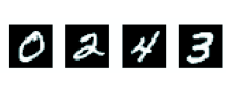
The problem we’re trying to solve here is to classify grayscale images of handwritten digits (28 × 28 pixels) into their 10 categories (0 through 9). We’ll use the MNIST dataset, a classic in the ML community, which has been around almost as long as the field itself and has been intensively studied. It’s a set of 60,000 training images, plus 10,000 test images, assembled by the National Institute of Standards and Technology (the NIST in MNIST) in the 1980s. You can think of “solving” MNIST as the “Hello World” of deep learning: it’s what you do to verify that your algorithms are working as expected. As you become a ML practitioner, you’ll see MNIST come up over and over again, in scientific papers, blog posts, and so on. You can see some MNIST samples in figure 2.1.

Note

In ML, a category in a classification problem is called a class. Data points are called samples. The class associated with a specific sample is called a label.

Sample MNIST digits

The MNIST dataset comes preloaded in Keras in a set of four arrays.

Listing 2.1: Loading the MNIST dataset in Keras

library(keras3)
.[.[train_images, train_labels], .[test_images, test_labels]] <-
  dataset_mnist()

train_images and train_labels form the training set, the data that the model will learn from. The model will then be tested on the test set, test_images and test_labels. The images are encoded as arrays, and the labels are an array of digits, ranging from 0 to 9. The images and labels have a one-to-one correspondence.

Let’s look at the training data:

str(train_images)

 int [1:60000, 1:28, 1:28] 0 0 0 0 0 0 0 0 0 0 ...

str(train_labels)

 int [1:60000(1d)] 5 0 4 1 9 2 1 3 1 4 ...

And here’s the test data:

str(test_images)

 int [1:10000, 1:28, 1:28] 0 0 0 0 0 0 0 0 0 0 ...

str(test_labels)

 int [1:10000(1d)] 7 2 1 0 4 1 4 9 5 9 ...

The workflow will be as follows. First we’ll feed the neural network the training data, train_images and train_labels. The network will then learn to associate images and labels. Finally, we’ll ask the network to produce predictions for test_images, and we’ll verify whether these predictions match the labels from test_labels.

Let’s build the network—again, remember that you aren’t expected to understand everything about this example yet.

Listing 2.2: The network architecture

model <- keras_model_sequential() |>
  layer_dense(512, activation = "relu") |>
  layer_dense(10, activation = "softmax")

The core building block of neural networks is the layer. You can think of a layer as a filter for data: some data goes in, and it comes out in a more useful form. Specifically, layers extract representations from the data fed into them—hopefully, representations that are more meaningful for the problem at hand. Most of deep learning consists of chaining together simple layers that will implement a form of progressive data distillation. A deep learning model is like a sieve for data processing, made of a succession of increasingly refined data filters: the layers.

Here, our model consists of a sequence of two Dense layers, which are densely connected (also called fully connected) neural layers. The second (and last) layer is a 10-way softmax classification layer, which means it will return an array of 10 probability scores (summing to 1). Each score will be the probability that the current digit image belongs to one of our 10 digit classes.

To make the model ready for training, we need to pick three more things, as part of the compilation step:

• A loss function—How the model will measure its performance on the training data and thus how it will steer itself in the right direction.
• An optimizer—The mechanism through which the model will update itself based on the training data it sees, to improve its performance.
• Metrics to monitor during training and testing—Here, we’ll only care about accuracy (the fraction of the images that were correctly classified).

The exact purpose of the loss function and the optimizer will be made clear throughout the next two chapters.

Listing 2.3: The compilation step

model |> compile(
  optimizer = "adam",
  loss = "sparse_categorical_crossentropy",
  metrics = "accuracy"
)

Before training, we’ll preprocess the data by reshaping it into the shape the model expects and scaling it so that all values are in the [0, 1] interval. Previously, our training images were stored in an array of shape (60000, 28, 28) of type integer with values in the [0, 255] interval. We transform it into a double array of shape (60000, 28 * 28) with values between 0 and 1.

Listing 2.4: Preparing the image data

train_images <- array_reshape(train_images, c(60000, 28 * 28))
train_images <- train_images / 255
test_images <- array_reshape(test_images, c(10000, 28 * 28))
test_images <- test_images / 255

Note that we use the array_reshape() function rather than the dim<-() function to reshape the array. We’ll explain why later, when we talk about tensor reshaping.

We’re now ready to train the model, which in Keras is done via a call to the model’s fit() method: we fit the model to its training data.

Listing 2.5: Fitting the model

fit(model, train_images, train_labels, epochs = 5, batch_size = 128)

Two quantities are displayed during training: the model’s loss on the training data and its accuracy on the training data. We quickly reach an accuracy of 0.989 (98.9%) on the training data.

Now that we have a trained model, we can use it to predict class probabilities for new digits: images that weren’t part of the training data, like those from the test set.

Listing 2.6: Using the model to make predictions

test_digits <- test_images[1:10, ]
predictions <- predict(model, test_digits)
str(predictions)

 num [1:10, 1:10] 0.000000198 0.0000000921 0.0000119322 0.9999227524 0.0000005135 ...

predictions[1, ]

 [1] 0.0000001980491788 0.0000000045636463 0.0000181329669431
 [4] 0.0006373987416737 0.0000000034133356 0.0000002556253662
 [7] 0.0000000000106126 0.9993394017219543 0.0000001938769429
[10] 0.0000042834572014

Each number of index i in that array corresponds to the probability that digit image test_digits[1] belongs to class i. This first test digit has the highest probability score (0.9993394, almost 1) at index 8, so according to our model, it must be a 7 (because the first position corresponds to digit “0”):

which.max(predictions[1,])

[1] 8

predictions[1, 8]

[1] 0.9993394

We can check that the test label agrees:

test_labels[1]

[1] 7

On average, how good is our model at classifying such never-before-seen digits? Let’s check by computing average accuracy over the entire test set.

Listing 2.7: Evaluating the model on new data

metrics <- evaluate(model, test_images, test_labels)
metrics$accuracy

[1] 0.9784

The test-set accuracy turns out to be 97.8%—that’s almost double the error rate of the training set (at 98.9% accuracy). This gap between training accuracy and test accuracy is an example of overfitting: the fact that ML models tend to perform worse on new data than on their training data. Overfitting is a central topic in chapter 5.

This concludes our first example. You just saw how you can build and train a neural network to classify handwritten digits in fewer than 20 lines of R code. In this chapter and the next, we’ll go into detail about every moving piece we just previewed and clarify what’s going on behind the scenes. You’ll learn about tensors, the data-storing objects going into the model; tensor operations, which layers are made of; and gradient descent, which allows your model to learn from its training examples.

2.2 Data representations for neural networks

In the previous example, we started from data stored in multidimensional arrays, also called tensors. In general, all current ML systems use tensors as their basic data structure. Tensors are fundamental to the field—so fundamental that the TensorFlow framework was named after them. So what’s a tensor?

At its core, a tensor is a container for data—usually numerical data. So, it’s a container for numbers. You may already be familiar with matrices, which are rank-2 tensors: tensors are a generalization of matrices to an arbitrary number of dimensions (note that in the context of tensors, a dimension is often called an axis).

R comes with a built-in tensor implementation: R arrays. Throughout this book, we’ll encounter a few other implementations of tensors: NumPy, TensorFlow, PyTorch, Jax, and Keras itself. To introduce the core ideas, we’ll start with R arrays and NumPy arrays.

NoteThe NumPy library

NumPy is a highly popular Python library for numerical computation. You will see it pop up frequently in your ML journey. It is rarely used to implement modern ML algorithms due to a lack of GPU and autodifferentiation support, but NumPy arrays are often used as a numerical data exchange format.

NumPy arrays also share common syntax and idioms with tensor objects from backend libraries like TensorFlow, Jax, and PyTorch, which you’ll encounter later in the book.

Don’t be confused by the “Py” in NumPy—it’s not just for Python users. NumPy arrays in R bring capabilities beyond base R arrays, such as

• A wider set of data types
• Modify-in-place semantics, giving us greater control over when array copies are made
• Flexible and convenient broadcasting behavior when working with multiple n-dimensional arrays (nd-arrays)
• A rich vocabulary for performing common tensor operations

Throughout this book, we’ll use both R arrays and NumPy arrays, writing in a macaronic blend that mixes idioms and functions, using the best each has to offer.

Note that any time we pass an R array to Keras, or to one of the deep-learning backends (TensorFlow, JAX, PyTorch), or to any Python function in R, the R array is automatically converted to a NumPy array. If you’re worried about the performance overhead of this, don’t be. The conversion is efficient and generally does not involve copying data: the created NumPy array points to the same underlying memory as the R array. Similarly, the Python functions called from R run at the same speed as when called from Python. This is because the reticulate package loads a full Python interpreter session and provides native access to it within R.

We can convert an R array to a NumPy array explicitly by calling np_array() or r_to_py(), and we can convert a NumPy array to an R array with as.array() or py_to_r(). To access the full NumPy API, we can import the "numpy" module in R like this:

np <- import("numpy")
np$sum(1:3)

[1] 6

Notice that the NumPy function returns an R object. To have the NumPy functions return NumPy arrays, import the module with convert = FALSE. Then we can explicitly convert the NumPy objects to R when we’re ready:

np <- import("numpy", convert = FALSE)
np$sum(1:3)

np.int64(6)

np$sum(1:3) |> np$square() |> py_to_r()

[1] 36

Going over the details of tensors might seem a bit abstract at first. But it’s well worth it: manipulating tensors will be the bread and butter of any ML code you write.

2.2.1 Scalars (rank-0 tensors)

A tensor that contains only one number is called a scalar (or scalar tensor, rank-0 tensor, or 0D tensor). R doesn’t have a data type to represent scalars (all numeric objects are vectors), but an R vector of length 1 is conceptually similar to a scalar.

In NumPy, a float32 or float64 number is a scalar tensor (or scalar array). We can display the number of axes of a NumPy tensor via the ndim attribute; a scalar tensor has 0 axes (ndim == 0). The number of axes of a tensor is also called its rank. Here’s a NumPy scalar:

x <- np$array(12)
x

array(12.)

x$ndim

0

2.2.2 Vectors (rank-1 tensors)

An array of numbers is called a vector (or rank-1 tensor or 1D tensor). A rank-1 tensor has exactly one axis. The following is an R array vector:

x <- as.array(c(12, 3, 6, 14, 7))
str(x)

 num [1:5(1d)] 12 3 6 14 7

dim(x)

[1] 5

And the same as a NumPy array:

x <- np_array(x)
x

array([12.,  3.,  6., 14.,  7.])

x$shape

(5,)

x$ndim

1

This vector has five entries and so is called a five-dimensional vector. Don’t confuse a 5D vector with a 5D tensor! A 5D vector has only one axis and has five dimensions along its axis, whereas a 5D tensor has five axes (and may have any number of dimensions along each axis). Dimensionality can denote either the number of entries along a specific axis (as in the case of our 5D vector) or the number of axes in a tensor (such as a 5D tensor), which can be confusing at times. In the latter case, it’s technically more correct to talk about a tensor of rank 5 (the rank of a tensor being the number of axes), but the ambiguous notation 5D tensor is common regardless.

2.2.3 Matrices (rank-2 tensors)

An array of vectors is a matrix (or rank-2 tensor or 2D tensor). A matrix has two axes (often referred to as rows and columns). We can visually interpret a matrix as a rectangular grid of numbers. This is a matrix:

x <- array(seq(2 * 3), dim = c(2, 3))
x

     [,1] [,2] [,3]
[1,]    1    3    5
[2,]    2    4    6

length(dim(x))

[1] 2

x <- np_array(x)
x

array([[1, 3, 5],
       [2, 4, 6]], dtype=int32)

x$ndim

2

The entries from the first axis are called the rows, and the entries from the second axis are called the columns. In the previous example, c(1, 3, 5) is the first row of x, and c(1, 2) is the first column.

2.2.4 Rank-3 tensors and higher-rank tensors

If we pack such matrices in a new array, we obtain a rank-3 tensor (or 3D tensor), which we can visually interpret as a cube of numbers. The following is a rank-3 tensor:

x <- array(seq(2 * 3 * 4), dim = c(4, 3, 2))
str(x)

 int [1:4, 1:3, 1:2] 1 2 3 4 5 6 7 8 9 10 ...

length(dim(x))

[1] 3

x

, , 1

     [,1] [,2] [,3]
[1,]    1    5    9
[2,]    2    6   10
[3,]    3    7   11
[4,]    4    8   12

, , 2

     [,1] [,2] [,3]
[1,]   13   17   21
[2,]   14   18   22
[3,]   15   19   23
[4,]   16   20   24

x <- np_array(x)
str(x)

<numpy.ndarray shape(4,3,2), dtype=int32>

x$ndim

3

x$shape

(4, 3, 2)

x

array([[[ 1, 13],
        [ 5, 17],
        [ 9, 21]],

       [[ 2, 14],
        [ 6, 18],
        [10, 22]],

       [[ 3, 15],
        [ 7, 19],
        [11, 23]],

       [[ 4, 16],
        [ 8, 20],
        [12, 24]]], dtype=int32)

Warning

Note that the print methods for the 3D R array and NumPy array make it seem like the elements are in a different order. They are not! This is only because NumPy by default prints using row-major order, whereas R prints using column-major order. See https://rstudio.github.io/reticulate/articles/arrays.html to learn more.

By packing (stacking) rank-3 tensors, we can create a rank-4 tensor, and so on. In deep learning, you’ll generally manipulate tensors with ranks 0 to 4, although you may go up to 5 if you process video data.

2.2.5 Key attributes

A tensor is defined by three key attributes:

• Number of axes (rank)—For instance, a rank-3 tensor has three axes, and a matrix has two axes. This is available from length(dim(x)) for R arrays and is also available as a tensor attribute, x$ndim, or via the accessor op_ndim(x) for tensor objects from libraries such as NumPy, JAX, TensorFlow, and PyTorch.

• Shape—This is a list of integers that describes how many dimensions the tensor has along each axis. For instance, the previous matrix example has shape (2, 3), and the rank-3 tensor example has shape (4, 3, 2). A vector has a shape with a single element, such as (5), whereas a scalar has an empty shape, (). We can get the shape of a tensor as an R list using op_shape(x).

• Data type (commonly called dtype in deep learning frameworks)— This is the type of the data contained in the tensor; R arrays are typically one of R’s built-in data types like double, integer, and logical. Tensors can support any type of homogeneous data type, and other tensor implementations also provide support for types like float16, float32, float64 (corresponding to R’s double), int32 (R’s integer type), uint8, and so on. In TensorFlow, you are also likely to come across string tensors. For R arrays, the type can be accessed with typeof(x); and for backend tensor objects, the dtype is typically available as a named attribute, x$dtype, or via op_dtype(x).

To make this more concrete, let’s look back at the data we processed in the MNIST example. This time, let’s load the data as NumPy arrays and do the preprocessing using NumPy:

.[.[train_images, train_labels], .[test_images, test_labels]] <-
1  dataset_mnist(convert = FALSE)

1

The .[<- method is provided by the dotty package and described in chapter 4.

Next, we display the number of axes of the tensor train_images, the ndim attribute:

op_ndim(train_images)

[1] 3

Here’s its shape:

op_shape(train_images)

shape(60000, 28, 28)

And this is its data type (dtype):

op_dtype(train_images)

[1] "uint8"

So what we have here is a rank-3 tensor of unsigned 8-bit integers. More precisely, it’s an array of 60,000 matrices of 28 × 28 integers. Each such matrix is a grayscale image with coefficients ranging from 0 to 255 (the range of values an unsigned 8-bit integer can represent).

Let’s display the fifth digit in this rank-3 tensor; see figure 2.2. Naturally, the corresponding label is just the integer 9:

train_labels@r[5]

np.uint8(9)

Listing 2.8: Displaying the fifth digit

digit <- train_images@r[5, , ] |> py_to_r() |>
  scales::rescale(to = c(0, 1), from = c(255, 0))
par(pty = "s", mar = c(1, 1, 1, 1))
plot(as.raster(digit), interpolate = FALSE)
box()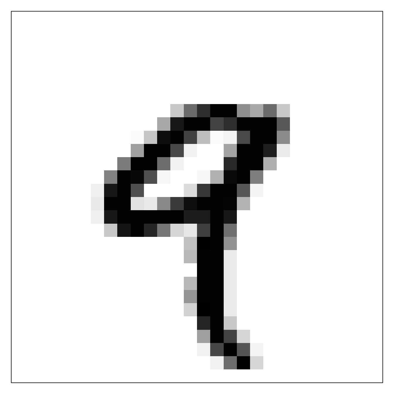

2.2.6 Manipulating NumPy tensors in R

In the previous example, we selected a specific digit alongside the first axis using the syntax train_images@r[i, , ]. Selecting specific elements in a tensor is called tensor slicing. Let’s look at the tensor-slicing operations you can do on NumPy arrays.

You will be able to do the same slicing operations on tensors from Jax, TensorFlow, and PyTorch later in the book. Throughout the book, we’ll use a combination of both R arrays and framework tensors.

In R, the [ method supports a rich set of behaviors for extracting subsets of an array, including slicing with 1D integer vectors, a combination of 1D integer vectors, _n_d integer arrays, and logical arrays. (For a great comprehensive guide to subsetting R arrays with [, check out https://adv-r.hadley.nz/subsetting.html#matrix-subsetting.)

Similarly, in Python, the [ method for NumPy arrays also supports a rich set of features, but the exact capabilities, idioms, and behaviors differ. From R, we can access both R-style and Python-style [ behaviors on tensors with x@r[] or x@py[].

One difference between the methods is that Python-style uses zero indexing, whereas R uses one-based indexing.

x <- np_array(1:10)
x@r[1]

np.int32(1)

x@py[1]

np.int32(2)

Another difference is that Python slices are exclusive of the slice end, whereas R’s are inclusive:

x@r[1:3]

array([1, 2, 3], dtype=int32)

x@py[1:3]

array([2, 3], dtype=int32)

The tensor @r[ method also brings some new capabilities over the base [ method for R arrays. For example, we can slice with open-ended ranges, using NA as a placeholder, which means “to the end of the array in that direction”:

x@r[NA:5]

array([1, 2, 3, 4, 5], dtype=int32)

x@r[6:NA]

array([ 6,  7,  8,  9, 10], dtype=int32)

Another difference between Tensor @r[ and base R Array’s [ is that missing axes in nd-arrays are implicitly filled in.

The following examples slice train_images along the first axis, select digits #10 to #99, and put them in an array of shape (90, 28, 28). These @r[ calls all produce the same result:

1my_slice <- train_images@r[10:99]
2my_slice <- train_images@r[10:99, , ]
3my_slice <- train_images@r[10:99, NA:NA, NA:NA]
4my_slice <- train_images@r[10:99, 1:28, 1:28]
my_slice$shape

1

The second and third axes are implicitly missing.

2

The second and third axes are explicitly missing.

3

The second and third axes slice start and end bounds are explicitly missing.

4

The second and third axes are the full axis bounds.

(90, 28, 28)

In general, we may select slices between any two indices along each tensor axis. For instance, to select 14 × 14 pixels in the bottom-right corner of all images, we would do this:

my_slice <- train_images@r[, 15:NA, 15:NA]
my_slice$shape

(60000, 14, 14)

We can also use newaxis or NULL to conveniently create size-1 axes. And the special symbol .. expands to “all the other axes”, making it easy to specify the last axes:

train_images$shape

(60000, 28, 28)

train_images@r[newaxis] |> _$shape

(1, 60000, 28, 28)

train_images@r[, newaxis] |> _$shape

(60000, 1, 28, 28)

train_images@r[.., newaxis] |> _$shape

(60000, 28, 28, 1)

train_images@r[.., newaxis, ] |> _$shape

(60000, 28, 1, 28)

It’s also possible to use negative indices.

CautionNegative indices

Negative indices used in @r[ have a different meaning from negative indices used in base R’s [ method. Negative numbers indicate a relative position from the end of the current axis. They do not mean “drop this element”, as they do in the base R array [ method.

For example:

x <- np_array(1:10)
x@r[-1]

np.int32(10)

x@r[-3:NA]

array([ 8,  9, 10], dtype=int32)

To crop the images to patches of 14 × 14 pixels centered in the middle, we can do this:

my_slice <- train_images@r[, 8:-8, 8:-8]
my_slice$shape

(60000, 14, 14)

That covers the basics of the @r[ method. To learn about other, more advanced features, check out the help page for ?op_subset and ?reticulate::py_get_item.

2.2.7 The notion of data batches

In general, the first axis in all data tensors you’ll come across in deep learning will be the samples axis. In the MNIST example, samples are images of digits.

In addition, deep learning models don’t process an entire dataset at once; rather, they break the data into small batches, or groups of samples with a fixed size. Concretely, here’s one batch of our MNIST digits, with a batch size of 128:

1batch <- train_images@r[1:128, , ]

1

Uses @r[ because train_images is a NumPy array.

And here’s the next batch:

batch <- train_images@r[129:256, , ]

And the _n_th batch:

n <- 3
ids <- seq(to = 128 * n, length.out = 128)
batch <- train_images@r[ids, , ]

When considering such a batch tensor, the first axis is called the batch axis (or batch dimension). You’ll frequently encounter this term when using Keras and other deep learning libraries.

2.2.8 Real-world examples of data tensors

Let’s make data tensors more concrete with a few examples similar to what you’ll encounter later. The data you’ll manipulate will almost always fall into one of the following categories:

• Vector data—Rank-2 tensors of shape (samples, features), where each sample is a vector of numerical attributes (“features”)
• Timeseries data or sequence data—Rank-3 tensors of shape (samples, timesteps, features), where each sample is a sequence (of length timesteps) of feature vectors
• Images—Rank-4 tensors of shape (samples, height, width, channels), where each sample is a 2D grid of pixels and each pixel is represented by a vector of values (“channels”)
• Video—Rank-5 tensors of shape (samples, frames, height, width, channels), where each sample is a sequence (of length frames) of images

2.2.8.1 Vector data

Vector data is one of the most common cases. In such a dataset, each single data point can be encoded as a vector, and thus a batch of data will be encoded as a rank-2 tensor (conceptually, a vector of vectors), where the first axis is the samples axis and the second axis is the features axis.

Let’s take a look at two examples:

• An actuarial dataset of people, where we consider each person’s age, gender, and income. Each person can be characterized as a vector of three values, and thus an entire dataset of 100,000 people can be stored in a rank-2 tensor of shape (100000, 3).

• A dataset of text documents, where we represent each document by the counts of how many times each word appears in it (out of a dictionary of 20,000 common words). Each document can be encoded as a vector of 20,000 values (one count per word in the dictionary), and thus an entire dataset of 500 documents can be stored in a tensor of shape (500, 20000).

2.2.8.2 Timeseries data or sequence data

Whenever time matters in your data (or the notion of sequence order), it makes sense to store it in a rank-3 tensor with an explicit time axis. Each sample can be encoded as a sequence of vectors (a rank-2 tensor), and thus a batch of data will be encoded as a rank-3 tensor (see figure 2.3).

A rank-3 timeseries data tensor

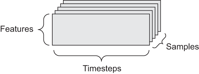
The time axis is always the second axis (index 1), by convention. Let’s look at a few examples:

• A dataset of stock prices—Every minute, we store the current price of the stock, the highest price in the past minute, and the lowest price in the past minute. Thus, every minute is encoded as a 3D vector, an entire day of trading is encoded as a matrix of shape (390, 3) (there are 390 minutes in a trading day), and 250 days’ worth of data can be stored in a rank-3 tensor of shape (250, 390, 3). Here, each sample would be one day’s worth of data.

• A dataset of tweets—We encode each tweet as a sequence of 280 characters out of an alphabet of 128 unique characters. In this setting, each character can be encoded as a binary vector of size 128 (an all-zeros vector except for a 1 entry at the index corresponding to the character). Then each tweet can be encoded as a rank-2 tensor of shape (280, 128), and a dataset of 1 million tweets can be stored in a tensor of shape (1000000, 280, 128).

2.2.8.3 Image data

Images typically have three dimensions: height, width, and color depth. Although grayscale images (like our MNIST digits) have only a single color channel and could thus be stored in rank-2 tensors, by convention, image tensors are always rank-3, with a 1D color channel for grayscale images. A batch of 128 grayscale images of size 256 × 256 could thus be stored in a tensor of shape (128, 256, 256, 1), and a batch of 128 color images could be stored in a tensor of shape (128, 256, 256, 3) (see figure 2.4).

A rank-4 image data tensor

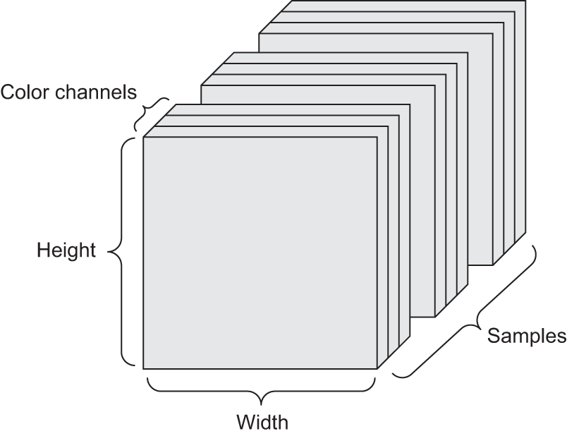
There are two conventions for the shapes of image tensors: the channels-last convention (which is standard in JAX and TensorFlow, as well as most other deep learning tools out there) and the channels-first convention (which is standard in PyTorch). The channels-last convention places the color-depth axis at the end: (samples, height, width, color_depth). Meanwhile, the channels-first convention places the color-depth axis right after the batch axis: (samples, color_depth, height, width). With the channels-first convention, the previous examples would become (128, 1, 256, 256) and (128, 3, 256, 256). The Keras API supports both formats.

2.2.8.4 Video data

Video data is one of the few types of real-world data for which you’ll need rank-5 tensors. A video can be understood as a sequence of frames, each frame being a color image. Because each frame can be stored in a rank-3 tensor (height, width, color_depth), a sequence of frames can be stored in a rank-4 tensor (frames, height, width, color_depth), and thus a batch of different videos can be stored in a rank-5 tensor of shape (samples, frames, height, width, color_depth).

For instance, a 60-second, 144 × 256 YouTube video clip sampled at 4 frames per second would have 240 frames. A batch of four such video clips would be stored in a tensor of shape (4, 240, 144, 256, 3). That’s a total of 106,168,320 values! If the dtype of the tensor were float32, then each value would be stored in 32 bits, so the tensor would represent 425 MB. Heavy! Videos you encounter in real life are much lighter because they aren’t stored in float32 and they’re typically compressed by a large factor (such as the MPEG format).

2.3 The gears of neural networks: Tensor operations

Just as any computer program can ultimately be reduced to a small set of binary operations on binary inputs (AND, OR, NOR, and so on), all transformations learned by deep neural networks can be reduced to a handful of tensor operations (or tensor functions) applied to tensors of numeric data. For instance, it’s possible to add tensors, multiply tensors, and so on.

In our initial example, we built our model by stacking Dense layers. A Keras layer instance looks like this:

layer_dense(units = 512, activation="relu")

This layer can be interpreted as a function that takes as input a matrix and returns another matrix—a new representation for the input tensor. Specifically, the function is as follows (where W is a matrix and b is a vector, both attributes of the layer):

output <- relu(matmul(input, W) + b)

Let’s unpack this. We have three tensor operations here:

• A tensor product (matmul) between the input tensor and a tensor named W
• An addition (+) between the resulting matrix and a vector b
• A relu operation: relu(x) is max(x, 0). “relu” stands for “REctified Linear Unit.”

Note

Although this section deals entirely with linear algebra expressions, you won’t find any mathematical notation in this book. We’ve found that mathematical concepts can be more readily mastered by programmers with no mathematical background if they’re expressed as short code snippets instead of mathematical equations. So we’ll use code throughout.

2.3.1 Element-wise operations

The relu operation and addition are element-wise operations: operations that are applied independently to each entry in the tensors being considered. This means these operations are highly amenable to massively parallel implementations (vectorized implementations, a term that comes from the vector processor supercomputer architecture from the 1970–1990 period). If we want to write a naive implementation of an element-wise operation on R arrays, we use a for loop, as in this naive implementation of an element-wise relu operation:

naive_relu <- function(x) {
1  stopifnot(is.array(x), length(dim(x)) == 2)
  for (i in 1:nrow(x))
    for (j in 1:ncol(x))
2      x[i, j] <- max(x[i, j], 0)
  x
}

1

x is a rank-2 tensor (a matrix).

2

R automatically makes a local copy of x in the function; the input x array is not modified in place.

We can do the same for addition:

naive_add <- function(x, y) {
  stopifnot(is.array(x), is.array(y),
1            length(dim(x)) == 2, dim(x) == dim(y))
  for (i in 1:nrow(x))
    for (j in 1:ncol(x))
      x[i, j]  <- x[i, j] + y[i, j]
  x
}

1

x and y are rank-2 R arrays.

On the same principle, we can do element-wise multiplication, subtraction, and so on.

In practice, when dealing with arrays, these operations are available as well-optimized built-in functions, which themselves delegate the heavy lifting to a Basic Linear Algebra Subprograms (BLAS) implementation. BLAS are low-level, highly parallel, efficient tensor-manipulation routines that are typically implemented in Fortran or C. So we can do the following element-wise operation, and it will be blazing fast:

1z <- x + y
2z <- pmax(z, 0.)

1

Element-wise addition

2

Element-wise relu

Let’s actually time the difference:

runif_array <- function(dim) {
  array(runif(prod(dim)), dim)
}

x <- runif_array(c(20, 100))
y <- runif_array(c(20, 100))

system.time({
  for (i in seq_len(10000)) {
    z <- x + y
    z <- pmax(z, 0)
  }
})[["elapsed"]]

[1] 0.145

This takes 0.14 seconds. Meanwhile, the naive version takes a stunning 8.37 seconds:

system.time({
  for (i in seq_len(10000)) {
    z <- naive_add(x, y)
    z <- naive_relu(z)
  }
})[["elapsed"]]

[1] 8.37

Likewise, when running JAX/TensorFlow/PyTorch code on a GPU, element-wise operations are executed via fully vectorized CUDA implementations that can best utilize the highly parallel GPU chip architecture.

2.3.2 Broadcasting

Our earlier naive implementation of naive_add only supports the addition of rank-2 tensors with identical shapes. But in the Dense layer introduced earlier, we added a rank-2 tensor with a vector. What happens with addition when the shapes of the two tensors being added differ?

When possible, and if there’s no ambiguity, the smaller tensor will be broadcasted to match the shape of the larger tensor. Broadcasting consists of two steps:

• Axes (called broadcast axes) are added to the smaller tensor to match the ndim of the larger tensor.
• The smaller tensor is repeated alongside these new axes to match the full shape of the larger tensor.

NoteBroadcasting vs. recycling

NumPy arrays implement broadcasting. Base R arrays have support for a limited form of broadcasting called recycling. Recycling is similar to broadcasting, but with an important difference: in NumPy, broadcasting occurs along axes, whereas in R, recycling happens only across a flattened array. This makes recycling harder to reason about with multidimensional arrays.

Clever uses of broadcasting in NumPy or recycling in R on nd-arrays can result in code that’s difficult to understand. To use broadcasting behavior for arrays of rank greater than 2, I recommend converting R arrays to NumPy arrays and making broadcast axes explicit by temporarily promoting the smaller-rank array with [newaxis] or op_expand_dims().

Let’s look at a concrete example. Consider X with shape (32, 10) and y with shape (10,):

1X <- np$random$random(shape(32, 10))
2y <- np$random$random(shape(10))

1

X is a random matrix with shape (32, 10).

2

y is a random vector with shape (10).

First we add an empty first axis to y, whose shape becomes (1, 10):

y <- y@r[newaxis, ..]
1str(y)

1

The shape of y is now (1, 10).

<numpy.ndarray shape(1,10), dtype=float64>

Then we repeat y 32 times alongside this new axis, so that we end up with a tensor Y with shape (32, 10), where Y[i, ] == y for i in seq(1, 32):

1Y <- np$tile(y, shape(32, 1))
Y$shape

1

Repeats y 32 times along the first axis to obtain Y with shape (32, 10).

(32, 10)

The equivalent of the np$tile() operation with R arrays would look like this:

y <- runif_array(c(10))
Y <- local({
  dim(y) <- c(1, 10)
1  y[rep(1, 32), ]
})

1

Repeats y 32 times along the first axis to obtain Y with shape (32, 10).

At this point, we can add X and Y because they have the same shape.

In terms of implementation, no new rank-2 tensor is created because that would be terribly inefficient. The repetition operation is entirely virtual: it happens at the algorithmic level rather than at the memory level. But thinking of the vector being repeated 32 times alongside a new axis is a helpful mental model. Here’s what a naive implementation would look like:

naive_add_matrix_and_vector <- function(x, y) {
1  stopifnot(length(dim(x)) == 2,
2            length(dim(y)) == 1,
            ncol(x) == dim(y))
  for (i in seq_len(dim(x)[1]))
    for (j in seq_len(dim(x)[2]))
      x[i, j] <- x[i, j] + y[j]
  x
}

1

x is a rank-2 array.

2

y is a rank-1 array.

With broadcasting on NumPy arrays (and backend framework tensors), we can generally apply two-tensor element-wise operations if one tensor has shape (a, b, … n, n + 1, … m) and the other has shape (n, n + 1, … m). The broadcasting will then automatically happen for axes a through n - 1.

The following example applies element-wise addition to two tensors of different shapes via broadcasting:

1x <- np_array(runif_array(c(64, 3, 32, 10)))
2y <- np_array(runif_array(c(32, 10)))
3z <- x + y

1

x is a random tensor with shape (64, 3, 32, 10).

2

y is a random tensor with shape (32, 10).

3

The output z has shape (64, 3, 32, 10) like x.

We can always make the implicit broadcast axes explicit with newaxis:

z_explicit <- x + y[newaxis, newaxis, ..]
all(py_to_r(z == z_explicit))

[1] TRUE

2.3.3 Tensor products

The tensor product, also called dot product or matmul (short for “matrix multiplication”) is one of the most common, most useful tensor operations. In R, a tensor product can be done using the %*% operator. This operator will automatically invoke np$matmul() for NumPy arrays or keras3::op_matmul() for backend tensors.

In mathematical notation, we’d note the operation with a dot (\cdot) (hence the name “dot product”):

x <- np_array(runif_array(32))
y <- np_array(runif_array(32))

1z <- x %*% y

np <- import("numpy", convert = FALSE)
2z <- np$matmul(x, y)

1

Takes the product between x and y.

2

This is equivalent.

z = x • y

Mathematically, what does the matmul operation do? Let’s start with the product of two vectors x and y. It’s computed as follows:

naive_vector_dot <- function(x, y) {
1  stopifnot(length(dim(x)) == 1,
            length(dim(y)) == 1,
            dim(x) == dim(y))
  z <- 0
  for (i in seq_along(x))
    z <- z + x[i] * y[i]
  z
}

1

x and y are 1D vectors of the same size.

You’ll have noticed that the product between two vectors is a scalar and that only vectors with the same number of elements are compatible for this operation.

We can also take the product between a matrix x and a vector y, which returns a vector where the coefficients are the products between y and the rows of x. We implement it as follows:

naive_matrix_vector_dot <- function(x, y) {
1  stopifnot(length(dim(x)) == 2,
2            length(dim(y)) == 1,
3            nrow(x) == dim(y))
4  z <- array(0, dim = nrow(x))
  for (i in 1:nrow(x))
    for (j in 1:ncol(x))
      z[i] <- z[i] + x[i, j] * y[j]
  z
}

1

x is a matrix.

2

y is a vector.

3

The 2nd dimension of x must equal the 1st dimension of y!

4

This operation returns a vector of 0s with as many rows as x

We can also reuse the code we wrote previously, which highlights the relationship between a matrix–vector product and a vector product:

naive_matrix_vector_dot <- function(x, y) {
  z <- array(0, dim = c(nrow(x)))
  for (i in 1:nrow(x))
    z[i] <- naive_vector_dot(x[i, ], y)
  z
}

Note that as soon as one of the two tensors has a rank (op_ndim()) greater than 1, matmul is no longer symmetric, which is to say that matmul(x, y) isn’t the same as matmul(y, x).

Of course, a tensor product generalizes to tensors with an arbitrary number of axes. The most common applications may be the product of two matrices. We can take the product of two matrices x and y (matmul(x, y)) if and only if dim(x)[2] == dim(y)[1]. The result is a matrix with shape (dim(x)[1], dim(y)[2]), where the coefficients are the vector products between the rows of x and the columns of y. Here’s the naive implementation:

naive_matrix_dot <- function(x, y) {
1  stopifnot(length(dim(x)) == 2,
            length(dim(y)) == 2,
2            ncol(x) == nrow(y))
3  z <- array(0, dim = c(nrow(x), ncol(y)))
4  for (i in 1:nrow(x))
5    for (j in 1:ncol(y)) {
      row_x <- x[i, ]
      column_y <- y[, j]
      z[i, j] <- naive_vector_dot(row_x, column_y)
    }
  z
}

1

x and y are matrices.

2

The 2nd dimension of x must equal the 1st dimension of y!

3

This operation returns a matrix of 0s with a specific shape.

4

Iterates over the rows of x …

5

… and over the columns of y.

To understand vector product shape compatibility, it helps to visualize the input and output tensors by aligning them as shown in figure 2.5.

Matrix product box diagram

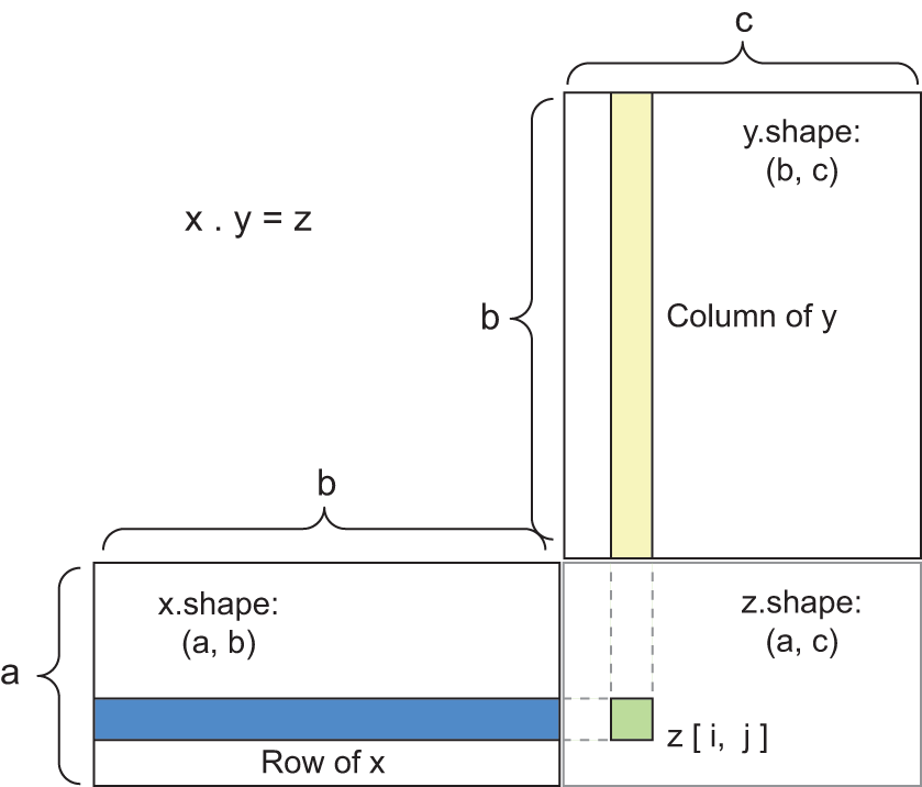
x, y, and z are pictured as rectangles (literal boxes of coefficients). Because the rows of x and the columns of y must have the same size, it follows that the width of x must match the height of y. If you go on to develop new ML algorithms, you’ll likely draw such diagrams often.

More generally, we can take the product between higher-dimensional tensors, following the same rules for shape compatibility as outlined earlier for the 2D case:

(a, b, c, d) • (d,) -> (a, b, c)
(a, b, c, d) • (d, e) -> (a, b, c, e)

And so on.

2.3.4 Tensor reshaping

A third type of tensor operation that’s essential to understand is tensor reshaping. Although it wasn’t used in the Dense layers in our first neural network example, we used it when we preprocessed the digits data before feeding it into our model:

train_images <- array_reshape(train_images, c(60000, 28 * 28))

Note that we use the array_reshape() function rather than the dim<-() function to reshape R arrays. This is so that the data is reinterpreted using row-major semantics (as opposed to R’s default column-major semantics), which is in turn compatible with the way the numerical libraries called by Keras (NumPy, TensorFlow, and so on) interpret array dimensions. You should always use the array_reshape() function when reshaping R arrays that will be passed to Keras.

Reshaping a tensor means rearranging its rows and columns to match a target shape. Naturally, the reshaped tensor has the same total number of coefficients as the initial tensor. Reshaping is best understood via simple examples:

x <- array(1:6)
x

[1] 1 2 3 4 5 6

array_reshape(x, dim = c(3, 2))

     [,1] [,2]
[1,]    1    2
[2,]    3    4
[3,]    5    6

array_reshape(x, dim = c(2, 3))

     [,1] [,2] [,3]
[1,]    1    2    3
[2,]    4    5    6

A special case of reshaping that’s commonly encountered is transposition. Transposing a matrix means exchanging its rows and its columns, so that x[i, ] becomes x[, i]:

x <- array(1:6, dim = c(3, 2))
x

     [,1] [,2]
[1,]    1    4
[2,]    2    5
[3,]    3    6

t(x)

     [,1] [,2] [,3]
[1,]    1    2    3
[2,]    4    5    6

2.3.5 Geometric interpretation of tensor operations

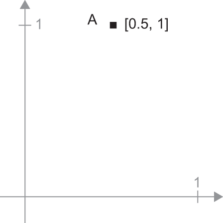
Because the contents of the tensors manipulated by tensor operations can be interpreted as coordinates of points in some geometric space, all tensor operations have a geometric interpretation. For instance, let’s consider addition. We’ll start with the following vector:

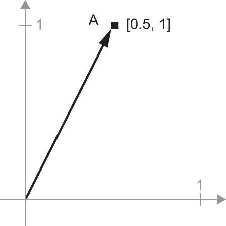
A = c(0.5, 1)

It’s a point in a 2D space (see figure 2.6). It’s common to picture a vector as an arrow linking the origin to the point, as shown in figure 2.7.

A point in a 2D space

A point in a 2D space pictured as an arrow

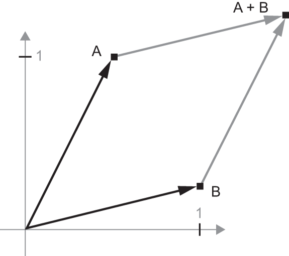
Let’s consider a new point, B = c(1, 0.25), which we’ll add to the previous one. This is done geometrically by chaining together the vector arrows, with the resulting location being the vector representing the sum of the previous two vectors (see figure 2.8). As you can see, adding a vector B to a vector A represents the action of copying point A in new location, whose distance and direction from the original point A are determined by the vector B. If we apply the same vector addition to a group of points in the plane (an object), we create a copy of the entire object in a new location (see figure 2.9). Tensor addition thus represents the action of translating an object (moving the object without distorting it) by a certain amount in a certain direction.

Geometric interpretation of the sum of two vectors

In general, elementary geometric operations, such as translation, rotation, scaling, skewing, and so on, can be expressed as tensor operations. Here are a few examples:

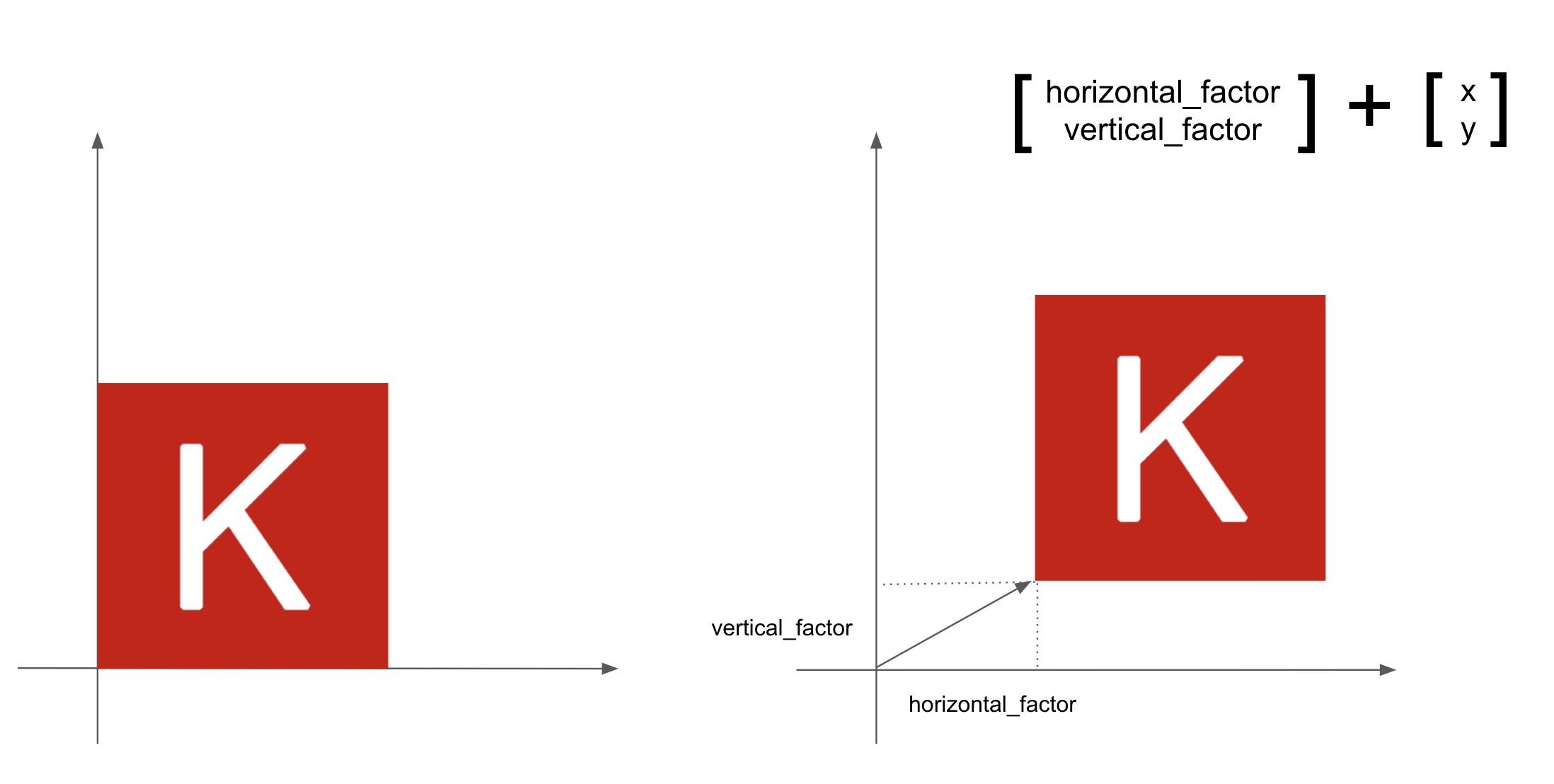
• Translation—As you just saw, adding a vector to a point will move this point by a fixed amount in a fixed direction. Applied to a set of points (such as a 2D object), this is called a translation (see figure 2.9).

2D translation as a vector addition

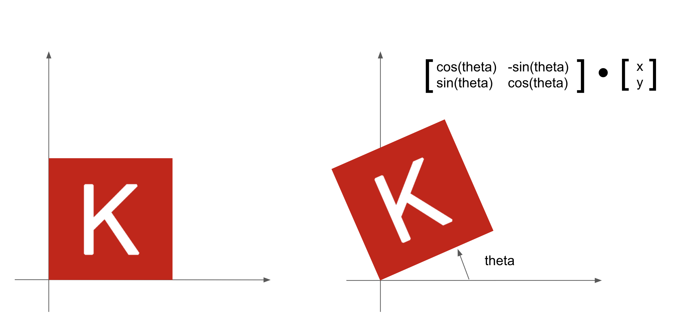
• Rotation—A counterclockwise rotation of a 2D vector by an angle theta (see figure 2.10) can be achieved via a product with a 2 × 2 matrix R = rbind(c(cos(theta), -sin(theta)), c(sin(theta), cos(theta))).

2D rotation (counterclockwise) as a matrix product

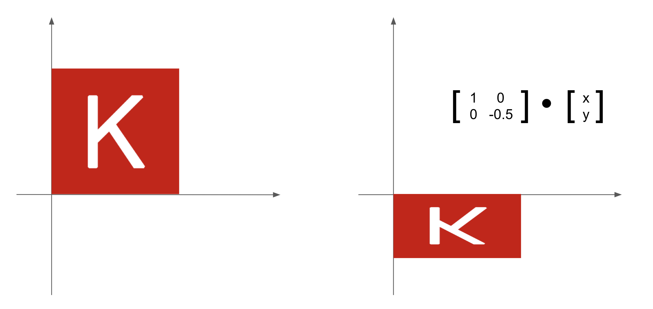
• Scaling—Vertical and horizontal scaling of the image (see figure 2.11) can be achieved via a product with a 2 × 2 matrix S = rbind(c(horizontal_factor, 0), c(0, vertical_factor)) (note that such a matrix is called a diagonal matrix because it only has nonzero coefficients in its diagonal going from top-left to bottom-right).

2D scaling as a matrix product

• Linear transform—A product with an arbitrary matrix implements a linear transform. Note that scaling and rotation, seen previously, are by definition linear transforms.

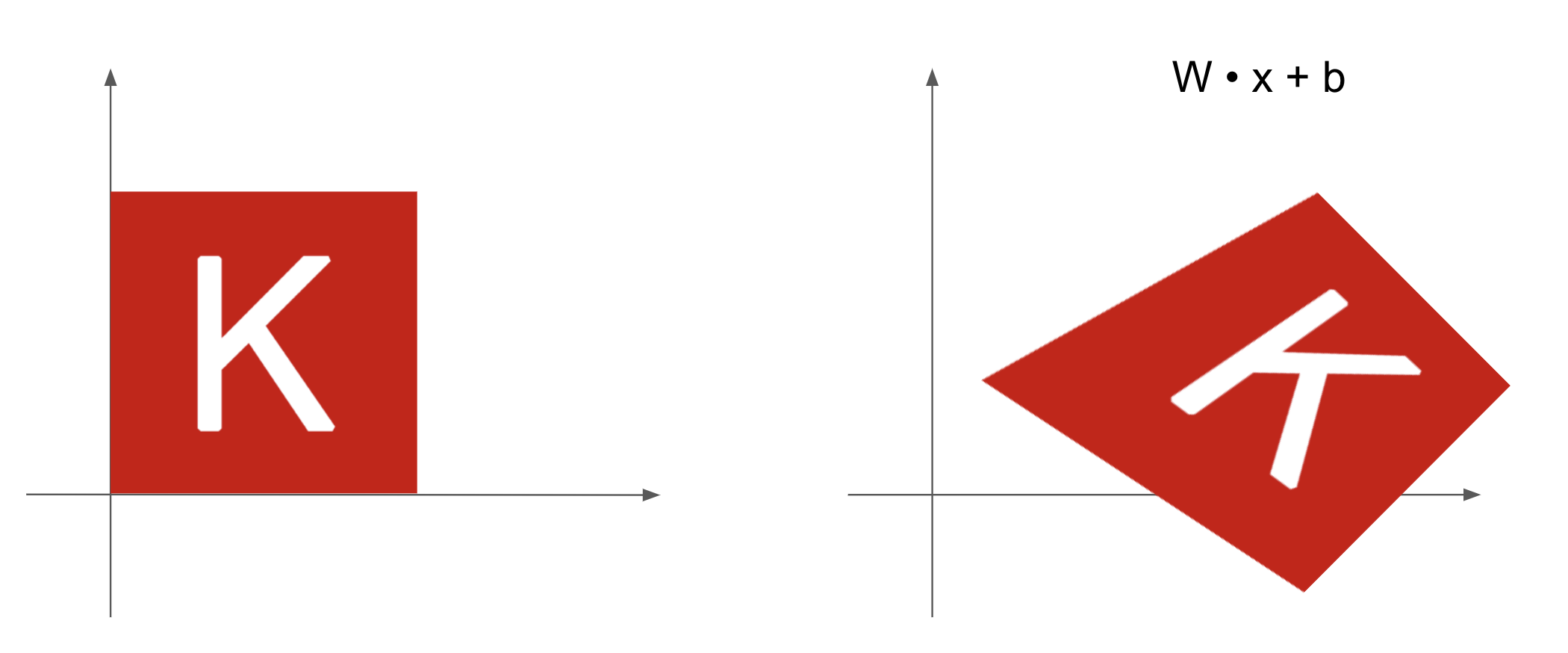
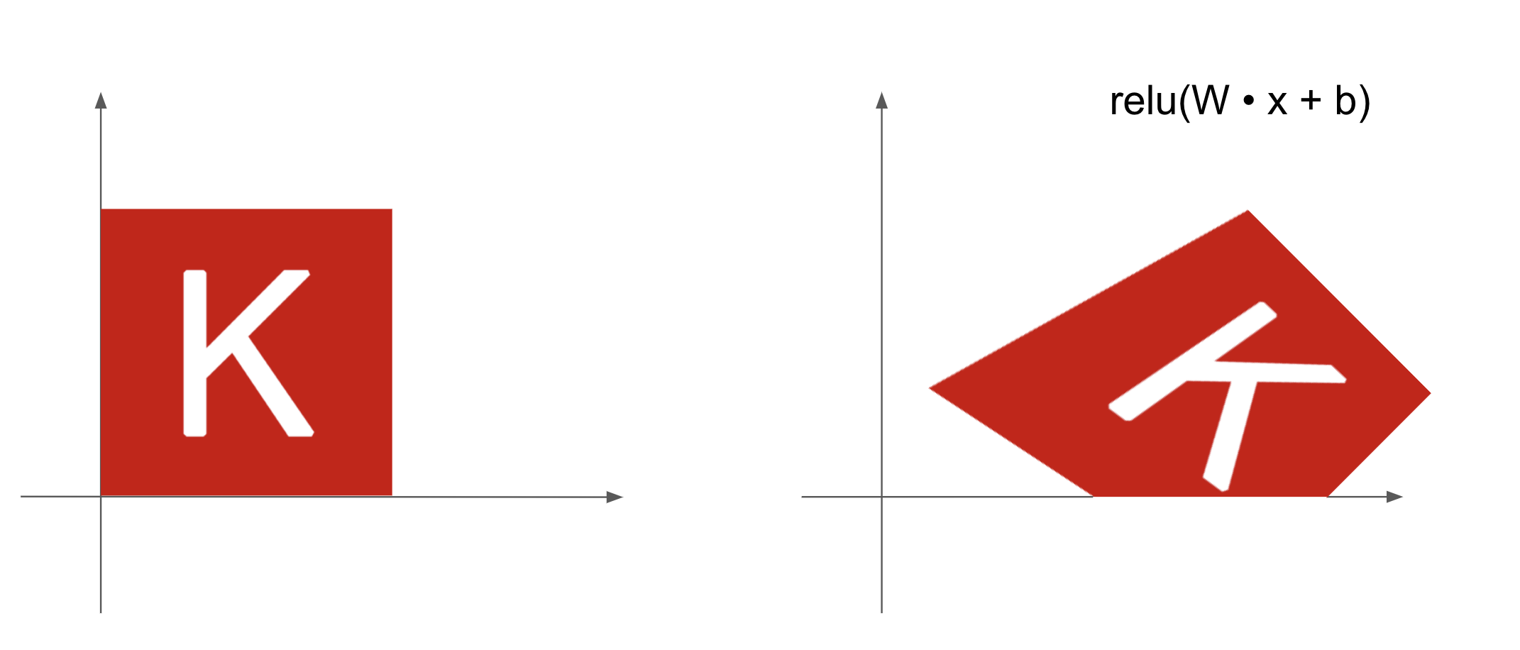
• Affine transform—The combination of a linear transform (achieved via a matrix product) and a translation (achieved via a vector addition) (see figure 2.12). As you have probably recognized, that’s exactly the y = x %*% W + b computation implemented by the Dense layer! A Dense layer without an activation function is an affine layer.

Affine transform in the plane

• Dense layer with relu activation—An important observation about affine transforms is that if we apply many of them repeatedly, we still end up with an affine transform (so we could just have applied that single affine transform in the first place). Let’s try it with two: affine2(affine1(x)) = W2 %*% (W1 %*% x + b1) + b2 = (W2 %*% W1) %*% x + (W2 %*% b1 + b2). That’s an affine transform where the linear part is the matrix W2 %*% W1 and the translation part is the vector W2 %*% b1 + b2. As a consequence, a multilayer neural network made entirely of Dense layers without activations would be equivalent to a single Dense layer. This “deep” neural network would be a linear model in disguise! This is why we need activation functions like relu (seen in action in figure 2.13). Thanks to activation functions, a chain of Dense layers can implement very complex, nonlinear geometric transformations, resulting in very rich hypothesis spaces for your deep neural networks. We cover this idea in more detail in the next chapter.

Affine transform followed by relu activation

2.3.6 A geometric interpretation of deep learning

You just learned that neural networks consist entirely of chains of tensor operations and that all of these tensor operations are just simple geometric transformations of the input data. It follows that you can interpret a neural network as a very complex geometric transformation in a high-dimensional space, implemented via a series of simple steps.

In 3D, the following mental image may prove useful. Imagine two sheets of colored paper: one red and one blue. Put one on top of the other. Now crumple them together into a small ball. That crumpled paper ball is your input data, and each sheet of paper is a class of data in a classification problem. What a neural network is meant to do is figure out a transformation of the paper ball that would uncrumple it to make the two classes cleanly separable again (see figure 2.14). With deep learning, this would be implemented as a series of simple transformations of the 3D space, such as those you could apply to the paper ball with your fingers, one movement at a time.

Uncrumpling a complicated manifold of data

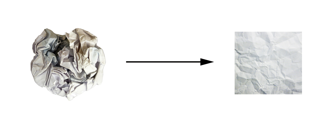
Uncrumpling paper balls is what ML is about: finding neat representations for complex, highly folded data manifolds in high-dimensional spaces (a manifold is a continuous surface, like our crumpled sheet of paper). At this point, you should have a pretty good intuition as to why deep learning excels at this: it takes the approach of incrementally decomposing a complicated geometric transformation into a long chain of elementary ones, which is pretty much the strategy a human would follow to uncrumple a paper ball. Each layer in a deep network applies a transformation that disentangles the data a little—and a deep stack of layers makes tractable an extremely complicated disentanglement process.

2.4 The engine of neural networks: Gradient-based optimization

As you saw in the previous section, each neural layer from our first model example transforms its input data as follows:

output <- relu(matmul(input, W) + b)

In this expression, W and b are tensors that are attributes of the layer. They’re called the weights or trainable parameters of the layer (the kernel and bias attributes, respectively). These weights contain the information the model has learned from its exposure to training data.

Initially, these weight matrices are filled with small random values (a step called random initialization). Of course, there’s no reason to expect that relu(matmul(input, W) + b), when W and b are random, will yield any useful representations. The resulting representations are meaningless—but they’re a starting point. What comes next is to gradually adjust these weights, based on a feedback signal. This gradual adjustment, also called training, is basically the learning that ML is all about.

This happens within what’s called a training loop, which works as follows. Repeat these steps in a loop until the loss seems sufficiently low:

1. Draw a batch of training samples x and corresponding targets y_true.
2. Run the model on x (a step called the forward pass) to obtain predictions y_pred.
3. Compute the loss of the model on the batch, a measure of the mismatch between y_pred and y_true.
4. Update all weights of the model in a way that slightly reduces the loss on this batch.

You’ll eventually end up with a model that has a very low loss on its training data: a low mismatch between predictions y_pred and expected targets y_true. The model has “learned” to map its inputs to correct targets. From afar, it may look like magic, but when you reduce it to elementary steps, it turns out to be simple.

Step 1 sounds easy enough—it’s just I/O code. Steps 2 and 3 are merely the application of a handful of tensor operations, so you could implement these steps purely from what you learned in the previous section. The difficult part is step 4: updating the model’s weights. Given an individual weight coefficient in the model, how can you compute whether the coefficient should be increased or decreased, and by how much?

One naive solution would be to freeze all weights in the model except the one scalar coefficient being considered and try different values for this coefficient. Let’s say the initial value of the coefficient is 0.3. After the forward pass on a batch of data, the model’s loss on that batch is 0.5. If you change the coefficient’s value to 0.35 and rerun the forward pass, the loss increases to 0.6. But if you lower the coefficient to 0.25, the loss falls to 0.4. In this case, it seems that updating the coefficient by -0.05 would help minimize the loss. This would have to be repeated for all model coefficients.

But such an approach would be horribly inefficient because you’d need to compute two forward passes (which are expensive) for every individual coefficient (of which there are many, usually at least a few thousand and potentially up to billions). Thankfully, there’s a much better approach: gradient descent.

Gradient descent is the optimization technique that powers modern neural networks. Here’s the gist of it. All of the functions used in our models (such as matmul and +) transform their input smoothly and continuously: if we look at z = x + y, for instance, a small change in y results in only a small change in z, and if we know the direction of the change in y, we can infer the direction of the change in z. Mathematically, we’d say these functions are differentiable. If we chain together such functions, the bigger function we obtain is still differentiable. In particular, this applies to the function that maps the model’s coefficients to the loss of the model on a batch of data: a small change of the model’s coefficients results in a small, predictable change of the loss value. This enables us to use a mathematical operator called the gradient to describe how the loss varies as we move the model’s coefficients in different directions. If we compute this gradient, we can use it to move the coefficients (all at once in a single update, rather than one at a time) in a direction that decreases the loss.

If you already know what differentiable means and what a gradient is, you can skip the next two sections. Otherwise, the following will help you understand these concepts.

2.4.1 What’s a derivative?

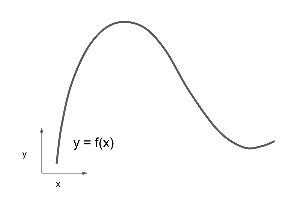
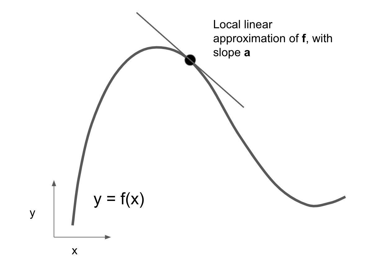
Consider a continuous, smooth function f(x) = y, mapping a number x to a new number y. We can use the function in figure 2.15 as an example.

A continuous, smooth function

Because the function is continuous, a small change in x can only result in a small change in y: that’s the intuition behind continuity. Let’s say we increase x by a small factor epsilon_x: this results in a small epsilon_y change to y, as shown in figure 2.16.

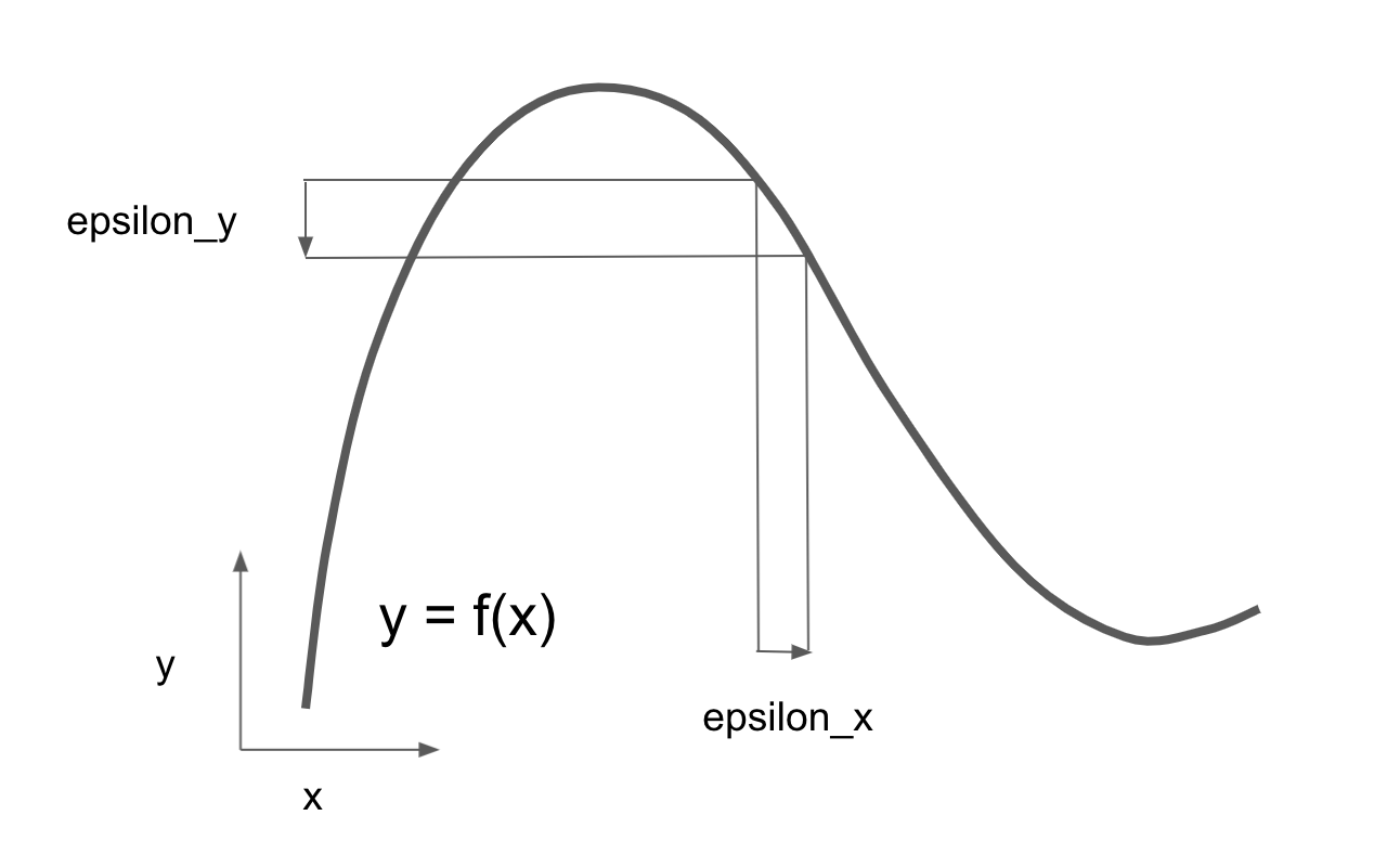
With a continuous function, a small change in x results in a small change in y

In addition, because the function is smooth (its curve doesn’t have any abrupt angles), when epsilon_x is small enough, around a certain point p, it’s possible to approximate f as a linear function of slope a, so that epsilon_y becomes a * epsilon_x:

f(x + epsilon_x) = y + a * epsilon_x

Obviously, this linear approximation is valid only when x is close enough to p.

The slope a is called the derivative of f in p. If a is negative, it means a small increase in x around p will result in a decrease of f(x), as shown in figure 2.17; and if a is positive, a small increase in x will result in an increase of f(x). Further, the absolute value of a (the magnitude of the derivative) tells us how quickly this increase or decrease will happen.

Derivative of f in p

For every differentiable function f(x) (differentiable means “can be derived”: for example, smooth, continuous functions can be derived), there exists a derivative function f'(x) that maps values of x to the slope of the local linear approximation of f in those points. For instance, the derivative of cos(x) is -sin(x), the derivative of f(x) = a * x is f'(x) = a, and so on.

Being able to derive functions is a very powerful tool when it comes to optimization, the task of finding values of x that minimize the value of f(x). If we’re trying to update x by a factor epsilon_x to minimize f(x) and we know the derivative of f, then your job is done: the derivative completely describes how f(x) evolves as we change x. If we want to reduce the value of f(x), we just need to move x a little in the opposite direction from the derivative.

2.4.2 Derivative of a tensor operation: The gradient

The function we were just looking at turned a scalar value x into another scalar value y: we could plot it as a curve in a 2D plane. Now, imagine a function that turns a pair of scalars (x, y) into a scalar value z: that would be a vector operation. We could plot it as a 2D surface in a 3D space (indexed by coordinates x, y, z). Likewise, we can imagine functions that take as input matrices, functions that take as input rank-3 tensors, etc.

The concept of derivation can be applied to any such function, as long as the surfaces they describe are continuous and smooth. The derivative of a tensor operation (or tensor function) is called a gradient. Gradients are just the generalization of the concept of derivatives to functions that take tensors as inputs. Remember how, for a scalar function, the derivative represents the local slope of the curve of the function? In the same way, the gradient of a tensor function represents the curvature of the multidimensional surface described by the function. It characterizes how the output of the function varies when its input parameters vary.

Let’s look at an example grounded in ML. Consider

• An input vector x (a sample in a dataset)
• A matrix W (the weights of a model)
• A target y_true (what the model should learn to associate with x)
• A loss function loss (meant to measure the gap between the model’s current predictions and y_true)

We can use W to compute a target candidate y_pred and then compute the loss, or mismatch, between the target candidate y_pred and the target y_true:

1y_pred = matmul(x, W)
2loss_value = loss(y_pred, y_true)

1

We use the model weights W to make a prediction for x.

2

We estimate how far off the prediction was.

Now, we’d like to use gradients to figure out how to update W to make loss_value smaller. How do we do that?

Given fixed inputs x and y_true, the previous operations can be interpreted as a function mapping values of W (the model’s weights) to loss values:

1loss_value = f(W)

1

f describes the curve (or high-dimensional surface) formed by loss values when W varies.

Let’s say the current value of W is W0. Then the derivative of f in the point W0 is a tensor grad(loss_value, W0) with the same shape as W, where each coefficient grad(loss_value, W0)[i, j] indicates the direction and magnitude of the change in loss_value we observe when modifying W0[i, j]. That tensor grad(loss_value, W0) is the gradient of the function f(W) = loss_value in W0, also called the gradient of loss_value with respect to W around W0.

NotePartial derivatives of a tensor operation

The tensor operation grad(f(W), W) (which takes as input a matrix W) can be expressed as a combination of scalar functions grad_ij(f(W), w_ij), each of which returns the derivative of loss_value = f(W) with respect to the coefficient W[i, j] of W, assuming all other coefficients are constant. grad_ij is called the partial derivative of f with respect to W[i, j].

Concretely, what does grad(loss_value, W0) represent? You saw earlier that the derivative of a function f(x) of a single coefficient can be interpreted as the slope of the curve of f. Likewise, grad(loss_value, W0) can be interpreted as the tensor describing the curvature of loss_value = f(W) around W0. Each partial derivative describes the curvature of f in a specific direction.

We just saw how, for a function f(x), we can reduce the value of f(x) by moving x a little in the opposite direction from the derivative. In much the same way, with a function f(W) of a tensor, we can reduce loss_value = f(W) by moving W in the opposite direction from the gradient, such as an update of W1 = W0 - step * grad(f(W0), W0) where step is a small scaling factor. That means going against the curvature, which intuitively should put us lower on the curve. Note that the scaling factor step is needed because grad(loss_value, W0) only approximates the curvature when we’re close to W0, so we don’t want to get too far from W0.

2.4.3 Stochastic gradient descent

Given a differentiable function, it’s theoretically possible to find its minimum analytically: it’s known that a function’s minimum is a point where the derivative is 0, so all we have to do is find all the points where the derivative goes to 0 and check for which of these points the function has the lowest value.

Applied to a neural network, that means finding analytically the combination of weight values that yields the smallest possible loss function. This can be done by solving the equation grad(f(W), W) = 0 for W. This is a polynomial equation of N variables, where N is the number of coefficients in the model. Although it would be possible to solve such an equation for N = 2 or N = 3, doing so is intractable for real neural networks, where the number of parameters is never less than a few thousand and can sometimes be in the billions.

Instead, we can use the four-step algorithm outlined at the beginning of this section: modify the parameters little by little based on the current loss value on a random batch of data. Because we’re dealing with a differentiable function, we can compute its gradient, which gives us an efficient way to implement step 4. If we update the weights in the opposite direction from the gradient, the loss will be a little less every time:

1. Draw a batch of training samples x and corresponding targets y_true.
2. Run the model on x to obtain predictions y_pred (this is called the forward pass).
3. Compute the loss of the model on the batch, a measure of the mismatch between y_pred and y_true.
4. Compute the gradient of the loss with regard to the model’s parameters (this is called the backward pass).
5. Move the parameters a little in the opposite direction from the gradient—for example, W = W - learning_rate * gradient—thus reducing the loss on the batch a bit. The learning rate (learning_rate here) is a scalar factor modulating the “speed” of the gradient descent process.

Easy enough! What we just described is called mini-batch stochastic gradient descent (mini-batch SGD). The term stochastic refers to the fact that each batch of data is drawn at random (stochastic is a scientific synonym of random). Figure 2.18 illustrates what happens in 1D when the model has only one parameter and we have only one training sample.

SGD down a 1D loss curve (one learnable parameter)

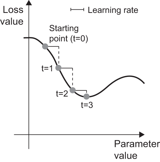
We can see intuitively that it’s important to pick a reasonable value for the learning_rate factor. If it’s too small, the descent down the curve will take many iterations, and it could get stuck in a local minimum. If learning_rate is too large, our updates may end up taking us to completely random locations on the curve.

Note that a variant of the mini-batch SGD algorithm would be to draw a single sample and target at each iteration, rather than drawing a batch of data. This would be true SGD (as opposed to mini-batch SGD). Alternatively, going to the opposite extreme, we could run every step on all data available, which is called batch gradient descent. Each update would then be more accurate, but far more expensive. The efficient compromise between these two extremes is to use mini-batches of reasonable size.

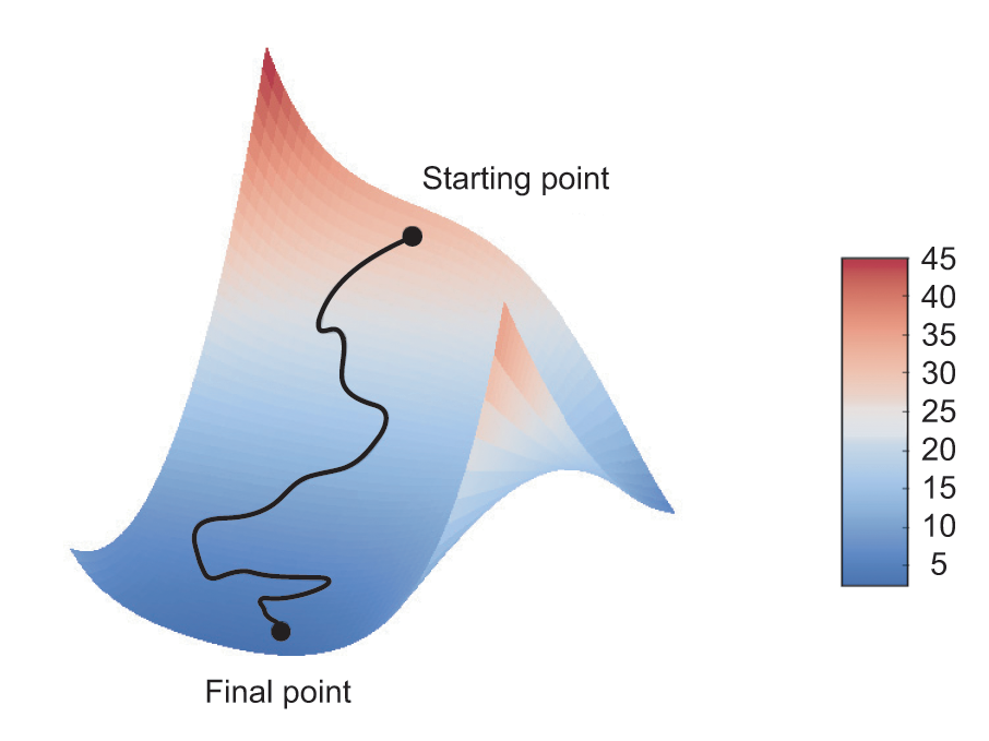
Although figure 2.18 illustrates gradient descent in a 1D parameter space, in practice, you’ll use gradient descent in highly dimensional spaces: every weight coefficient in a neural network is a free dimension in the space, and there may be tens of thousands or even millions of them. To help you build intuition about loss surfaces, you can also visualize gradient descent along a 2D loss surface, as shown in figure 2.19. But you can’t visualize what the actual process of training a neural network looks like—it’s impossible to represent a 1,000,000-dimensional space in a way that makes sense to humans. As such, it’s good to keep in mind that the intuitions you develop through these low-dimensional representations may not always be accurate in practice. This has historically been a source of problems in deep learning research.

Gradient descent down a 2D loss surface (two learnable parameters)

Additionally, there are multiple variants of SGD that take previous weight updates into account when computing the next weight update, rather than just looking at the current gradient values. For instance, there is SGD with momentum, as well as Adagrad, RMSprop, and several others. Such variants are known as optimization methods or optimizers. In particular, the concept of momentum, which is used in many of these variants, deserves your attention. Momentum addresses two problems with SGD: convergence speed and local minima. Consider figure 2.20, which shows the curve of a loss as a function of a model parameter.

A local minimum and a global minimum

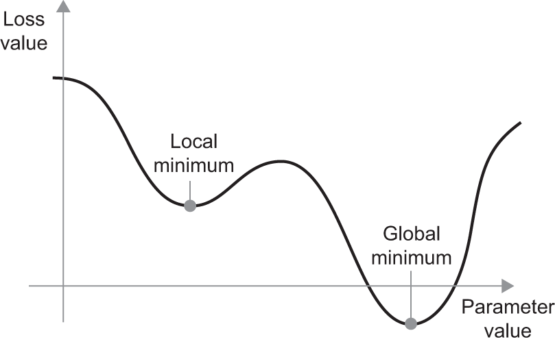
As you can see, around a certain parameter value, there is a local minimum: around that point, moving left would result in the loss increasing, but so would moving right. If the parameter under consideration were being optimized via SGD with a small learning rate, then the optimization process would get stuck at the local minimum instead of making its way to the global minimum.

We can avoid such problems by using momentum, which draws inspiration from physics. A useful mental image here is to think of the optimization process as a small ball rolling down the loss curve. If it has enough momentum, the ball won’t get stuck in a ravine and will end up at the global minimum. Momentum is implemented by moving the ball at each step based not only on the current slope value (current acceleration) but also on the current velocity (resulting from past acceleration). In practice, this means updating the parameter w based not only on the current gradient value but also on the previous parameter update, such as in this naive implementation:

past_velocity <- 0
1momentum <- 0.1
2while (loss > 0.01) {
  .[w, loss, gradient] <- get_current_parameters()
  velocity <- past_velocity * momentum - learning_rate * gradient
  w <- w + momentum * velocity - learning_rate * gradient
  past_velocity <- velocity
  update_parameter(w)
}

1

Constant momentum factor

2

Optimization loop

2.4.4 Chaining derivatives: The Backpropagation algorithm

In the previously discussed algorithm, we casually assumed that because a function is differentiable, we can easily compute its gradient. But is that true? How can we compute the gradient of complex expressions in practice? In our two-layer network example, how can we get the gradient of the loss with regard to the weights? That’s where the Backpropagation algorithm comes in.

2.4.4.1 The chain rule

Backpropagation is a way to use the derivative of simple operations (such as addition, relu, and tensor products) to easily compute the gradient of arbitrarily complex combinations of these atomic operations. Crucially, a neural network consists of many tensor operations chained together, each of which has a simple, known derivative. For instance, the model from our first example can be expressed as a function parameterized by the variables W1, b1, W2, and b2 (belonging to the first and second Dense layers, respectively), involving the atomic operations matmul, relu, softmax, and +, as well as our loss function, loss, which are all easily differentiable:

loss_value <- loss(
  y_true,
  softmax(matmul(relu(matmul(inputs, W1) + b1), W2) + b2)
)

Calculus tells us that such a chain of functions can be derived using the following identity, called the chain rule. Consider two functions f and g, as well as the composed function fg such that y = fg(x) == f(g(x)):

fg <- function(x) {
  x1 <- g(x)
  y <- f(x1)
  y
}

Then the chain rule states that grad(y, x) == grad(y, x1) * grad(x1, x). This enables us to compute the derivative of fg as long as we know the derivatives of f and g. The chain rule is called this because when we add more intermediate functions, it starts to look like a chain:

fghj <- function(x) {
  x1 <- j(x)
  x2 <- h(x1)
  x3 <- g(x2)
  y <- f(x3)
  y
}

grad(y, x) == (grad(y, x3) * grad(x3, x2) * grad(x2, x1) * grad(x1, x))

Applying the chain rule to the computation of the gradient values of a neural network gives rise to an algorithm called Backpropagation. Let’s see how that works, concretely.

2.4.4.2 Automatic differentiation with computation graphs

A useful way to think about backpropagation is in terms of computation graphs. A computation graph is the data structure at the heart of the deep learning revolution. It’s a directed acyclic graph of operations—in our case, tensor operations. For instance, figure 2.21 is the graph representation of our first model.

The computation graph representation of our two-layer model

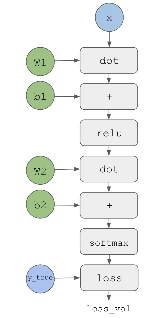
Computation graphs have been an extremely successful abstraction in computer science because they enable us to treat computation as data: a computable expression is encoded as a machine-readable data structure that can be used as the input or output of another program. For instance, you could imagine a program that receives a computation graph and returns a new computation graph that implements a large-scale distributed version of the same computation—this would mean you could distribute any computation without having to write the distribution logic yourself. Or imagine a program that receives a computation graph and can automatically generate the derivative of the expression it represents. It’s much easier to do these things if your computation is expressed as an explicit graph data structure rather than, say, lines of ASCII characters in a .R file.

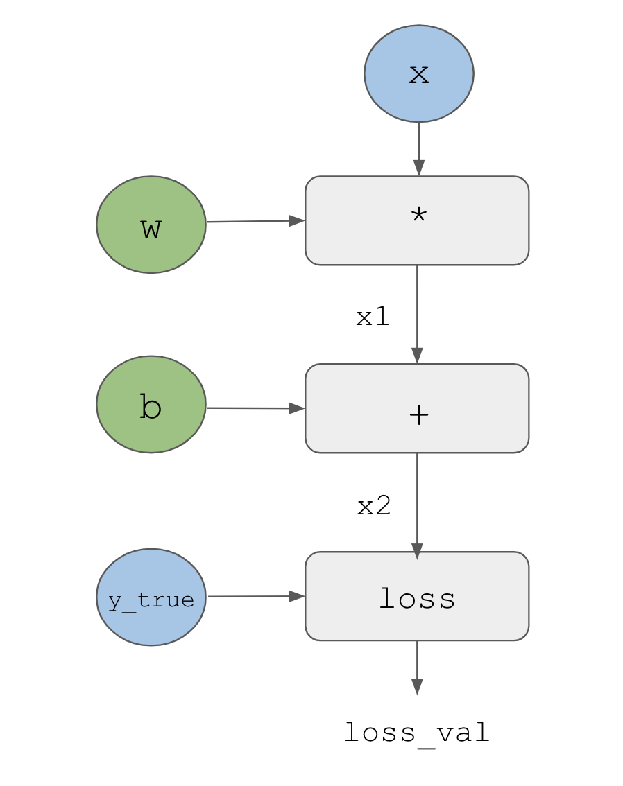
To explain backpropagation clearly, let’s look at a really basic example of a computation graph, shown in figure 2.22. We’ll consider a simplified version of the graph in figure 2.21, where we have only one linear layer and all variables are scalar. We’ll take two scalar variables w and b and a scalar input x and apply some operations to them to combine into an output y. Finally, we’ll apply an absolute value error loss function: loss_val = abs(y_true - y). Because we want to update w and b in a way that will minimize loss_val, we are interested in computing grad(loss_val, b) and grad(loss_val, w).

A basic example of a computation graph

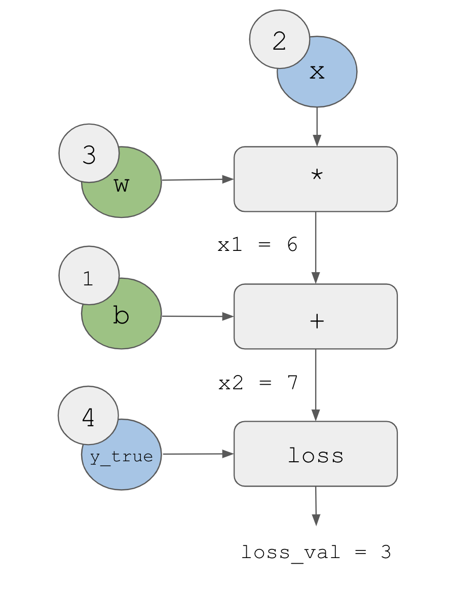
Let’s set concrete values for the “input nodes” in the graph—that is, the input x, the target y_true, w, and b (figure 2.23). We propagate these values to all nodes in the graph, from top to bottom, until we reach loss_val. This is the forward pass.

Running a forward pass

Now let’s “reverse” the graph: for each edge in the graph going from A to B, we will create an opposite edge from B to A and ask, “How much does B vary when A varies?” That is, what is grad(B, A)? We’ll annotate each inverted edge with this value (figure 2.24). This backward graph represents the backward pass.

Running a backward pass

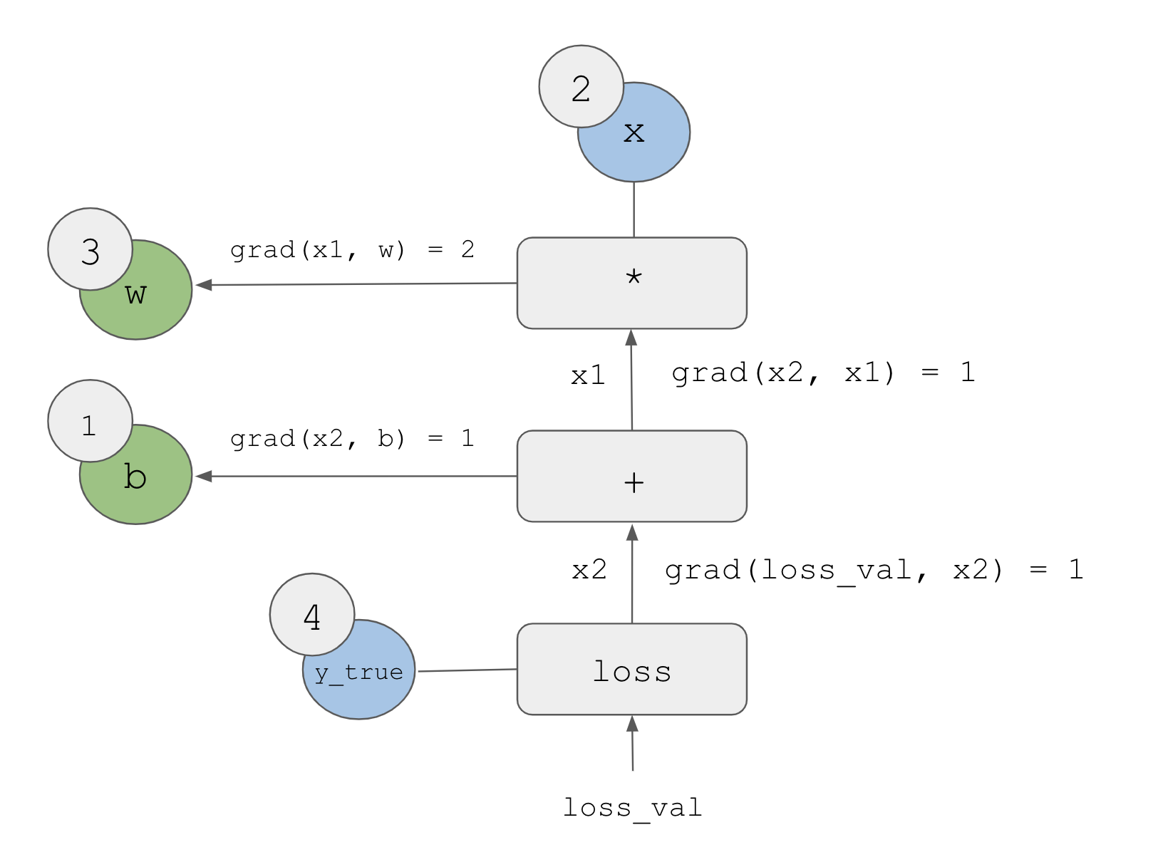
We have

• grad(loss_val, x2) = 1 because as x2 varies by an amount epsilon, loss_val = abs(4 - x2) varies by the same amount
• grad(x2, x1) = 1 because as x1 varies by an amount epsilon, x2 = x1 + b = x1 + 1 varies by the same amount
• grad(x2, b) = 1 because as b varies by an amount epsilon, x2 = x1 + b = 6 + b varies by the same amount
• grad(x1, w) = 2 because as w varies by an amount epsilon, x1 = x * w = 2 * w varies by 2 * epsilon

What the chain rule says about this backward graph is that we can obtain the derivative of a node with respect to another node by multiplying the derivatives for each edge along the path linking the two nodes. For instance, grad(loss_val, w) = grad(loss_val, x2) * grad(x2, x1) * grad(x1, w) (see figure 2.25).

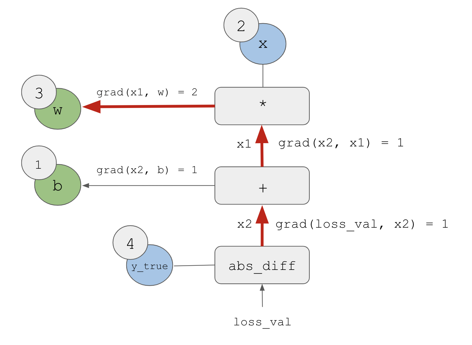
Path from loss_val to w in the backward graph

By applying the chain rule to our graph, we obtain what we were looking for:

• grad(loss_val, w) = 1 * 1 * 2 = 2
• grad(loss_val, b) = 1 * 1 = 1

Note

If there are multiple paths linking the two nodes of interest a and b in the backward graph, we will obtain grad(b, a) by summing the contributions of all the paths.

And with that, you just saw backpropagation in action! Backpropagation is simply the application of the chain rule to a computation graph. There’s nothing more to it. Backpropagation starts with the final loss value and works backward from the top layers to the bottom layers, computing the contribution that each parameter had in the loss value. That’s where the name “backpropagation” comes from: we “back propagate” the loss contributions of different nodes in a computation graph.

Nowadays, people implement neural networks in modern frameworks that are capable of automatic differentiation, such as JAX, TensorFlow, and PyTorch. Automatic differentiation is implemented using the kind of computation graph previously presented and makes it possible to retrieve the gradients of arbitrary compositions of differentiable tensor operations without doing any extra work besides writing down the forward pass. When I (François) wrote my first neural networks in C in the 2000s, I had to write my gradients by hand. Now, thanks to modern automatic differentiation tools, you’ll never have to implement backpropagation yourself. Consider yourself lucky!

2.5 Looking back at our first example

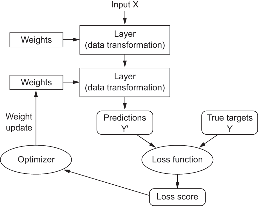
You’re nearing the end of this chapter, and you should now have a general understanding of what’s going on behind the scenes in a neural network. What was a magical black box at the start of the chapter has turned into a clearer picture, as illustrated in figure 2.26: the model, composed of layers that are chained together, maps the input data to predictions. The loss function then compares these predictions to the targets, producing a loss value: a measure of how well the model’s predictions match what was expected. The optimizer uses this loss value to update the model’s weights.

Relationship between the network, layers, loss function, and optimizer

Let’s go back to the first example and review each piece of it in the light of what you’ve learned in the previous sections. This time, we’ll do the preprocessing using NumPy instead of base R arrays.

This was the input data:

.[.[train_images, train_labels], .[test_images, test_labels]] <-
  dataset_mnist(convert = FALSE)

preprocess_images <- function(images) {
  images <- images$
    reshape(shape(nrow(images), 28 * 28))$
    astype("float32")
  images / 255
}

train_images <- train_images |> preprocess_images()
test_images <- test_images |> preprocess_images()
str(named_list(train_images,  test_images))

List of 2
 $ train_images: <numpy.ndarray shape(60000,784), dtype=float32>
 $ test_images : <numpy.ndarray shape(10000,784), dtype=float32>

Now you understand that the input images are stored in 8-bit unsigned integer NumPy tensors, which are here converted to float32 tensors with shapes (60000, 784) (training data) and (10000, 784) (test data), respectively, and rescaled from [0, 255] to [0, 1].

This was our model:

model <- keras_model_sequential() |>
  layer_dense(units = 512, activation = "relu") |>
  layer_dense(units = 10, activation = "softmax")

Now you understand that this model consists of a chain of two Dense layers, that each layer applies a few simple tensor operations to the input data, and that these operations involve weight tensors. Weight tensors, which are attributes of the layers, are where the knowledge of the model persists.

This was the model-compilation step:

model |> compile(
  optimizer = "adam",
  loss = "sparse_categorical_crossentropy",
  metrics = "accuracy"
)

Now you understand that "sparse_categorical_crossentropy" is the loss function that’s used as a feedback signal for learning the weight tensors, which the training phase will attempt to minimize. You also know that this reduction of the loss happens via mini-batch SGD. The exact rules governing a specific use of gradient descent are defined by the "adam" optimizer passed as the first argument.

Finally, this was the training loop:

fit(model, train_images, train_labels, epochs = 5, batch_size = 128)

Now you understand what happens when you call fit: the model will iterate over the training data in mini-batches of 128 samples, 5 times (each iteration over all the training data is called an epoch). For each batch, the model will compute the gradient of the loss with regard to the weights (using the Backpropagation algorithm, which derives from the chain rule in calculus) and move the weights in the direction that will reduce the value of the loss for this batch.

After these 5 epochs, the model will have performed 2,345 gradient updates (469 per epoch), and its loss will be sufficiently low that it can classify handwritten digits with high accuracy.

At this point, you know most of what there is to know about neural networks. Let’s prove it by reimplementing a simplified version of that first example step by step, using only low-level operations.

2.5.1 Reimplementing our first example from scratch

What’s better to demonstrate full, unambiguous understanding than to implement everything from scratch? Of course, what “from scratch” means here is relative: we won’t reimplement basic tensor operations, and we won’t implement backpropagation. But we’ll go to such a low level that each computation step will be made explicit.

Don’t worry if you don’t understand every detail in this example. The next chapter will dive into the Keras API in more detail. For now, just try to follow the gist of what’s going on—this example is meant to help crystallize your understanding of the mathematics of deep learning using a concrete implementation. Let’s go!

2.5.1.1 A simple Dense class

You learned earlier that the Dense layer implements the following input transformation, where W and b are model parameters and activation is an element-wise function (usually relu):

output <- activation(matmul(input, W) + b)

Let’s implement a simple R class NaiveDense that creates two Keras variables W and b and exposes a call() method that applies the previous transformation:

layer_naive_dense <- function(input_size, output_size, activation = NULL) {
1  self <- new.env(parent = emptyenv())
  attr(self, "class") <- "NaiveDense"

  self$activation <- activation

2  self$W <- keras_variable(shape = shape(input_size, output_size),
                           initializer = "uniform", dtype = "float32")

3  self$b <- keras_variable(shape = shape(output_size),
                           initializer = "zeros", dtype = "float32")

4  self$weights <- list(self$W, self$b)

5  self$call <- function(inputs) {
    x <- (inputs %*% self$W) + self$b
    if (is.function(self$activation))
      x <- self$activation(x)
    x
  }

  self
}

1

Uses an R environment so we can maintain state.

2

Creates a matrix W of shape (input_size, output_size), initialized with random values drawn from a uniform distribution.

3

Creates a vector b of shape (output_size), initialized with zeros.

4

Convenience for retrieving the layer’s weights.

5

Applies the forward pass.

2.5.1.2 A simple Sequential class

Now, let’s create a NaiveSequential class to chain these layers. It wraps a list of layers and exposes a call() method that simply calls the underlying layers on the inputs, in order. It also features a weights property to easily keep track of the layers’ parameters:

naive_sequential_model <- function(layers) {
  self <- new.env(parent = emptyenv())
  attr(self, "class") <- "NaiveSequential"

  self$layers <- layers

  self$weights <- unlist(lapply(layers, `[[`, "weights"))

  self$call <- function(inputs) {
    x <- inputs
    for (layer in self$layers)
      x <- layer$call(x)
    x
  }

  self
}

Using this NaiveDense class and this NaiveSequential class, we can create a mock Keras model:

model <- naive_sequential_model(list(
  layer_naive_dense(input_size = 28 * 28, output_size = 512,
                    activation = op_relu),
  layer_naive_dense(input_size = 512, output_size = 10,
                    activation = op_softmax)
))
stopifnot(length(model$weights) == 4)

2.5.1.3 A batch generator

Next, we need a way to iterate over the MNIST data in mini-batches. Let’s use a generator to make this easy:

new_batch_generator <- function(images, labels, batch_size = 128) {
  stopifnot(nrow(images) == nrow(labels))
  next_start <- 1

1  function(exhausted = NULL) {
    start <- next_start
    if (start > nrow(images))
2      return(exhausted)

    end <- start + batch_size - 1
3    end <- min(end, nrow(images))

    next_start <<- end + 1
    list(images = images@r[start:end, ..],
         labels = labels@r[start:end, ..])
  }
}

1

Returns a function that returns the next batch every time it’s called

2

The generator is finished.

3

The last batch may be smaller.

2.5.2 Running one training step

The most difficult part of the process is the “training step”: updating the model’s weights after running it on a single batch of data. We need to

• Compute the predictions of the model for the images in the batch
• Compute the loss value for these predictions given the actual labels
• Compute the gradient of the loss with regard to the model’s weights
• Move the weights by a small amount in the direction opposite to the gradient

Listing 2.9: A single step of training

one_training_step <- function(model, images_batch, labels_batch) {
1  predictions <- model$call(images_batch)
  loss <- op_sparse_categorical_crossentropy(labels_batch, predictions)
  average_loss <- op_mean(loss)
2  gradients <- get_gradients_of_loss_wrt_weights(loss, model$weights)
3  update_weights(gradients, model$weights)
  loss
}

1

Runs the forward pass

2

Computes the gradient of the loss with regard to the weights. The output gradients is a list in which each entry corresponds to a weight from the model$weights list. We haven’t defined this function yet!

3

Updates the weights using the gradients. We haven’t defined this function yet!

2.5.2.1 The weight update step

As you already know, the purpose of the “weight update” step (represented by the update_weights() function) is to move the weights a bit in a direction that will reduce the loss on this batch. The magnitude of the move is determined by the learning rate, typically a small quantity. The simplest way to implement this update_weights() function is to subtract gradient * learning_rate from each weight:

learning_rate <- 1e-3

update_weights <- function(gradients, weights) {
1  Map(\(w, g) w$assign(w - g * learning_rate),
      weights, gradients)
}

1

Assigns a new value to the variable, in place.

In practice, you will almost never implement a weight update step like this by hand. Instead, you will use an Optimizer instance from Keras—like this:

optimizer <- optimizer_sgd(learning_rate = 1e-3)

update_weights <- function(gradients, weights) {
  optimizer$apply(gradients, weights)
}

2.5.2.2 Gradient computation

Now we’re missing just one thing: gradient computation (represented by the get_gradients_of_loss_wrt_weights() function in listing 2.9). In the previous section, we outlined how to use the chain rule to obtain the gradients of a chain of functions given their individual derivatives, a process known as backpropagation. We could reimplement backpropagation from scratch here, but that would be cumbersome, especially because we’re using a softmax operation and a cross-entropy loss, which have fairly verbose derivatives.

Instead, we can rely on the automatic differentiation mechanism that’s built into one of the low-level frameworks supported by Keras, such as TensorFlow, JAX, or PyTorch. For the sake of the example, let’s go with TensorFlow here. You’ll learn more about TensorFlow, JAX, and PyTorch in the next chapter.

The API through which we can use TensorFlow’s automatic differentiation capabilities is the tf$GradientTape object. It’s a context scope that will “record” the tensor operations that run inside it, in the form of a computation graph (sometimes called a tape). This graph can then be used to retrieve the gradient of any scalar value with respect to any set of input values:

library(tensorflow)

1x <- tf$zeros(shape = shape())
2with(tf$GradientTape() %as% tape, {
3  y <- 2 * x + 3
})
4grad_of_y_wrt_x <- tape$gradient(y, x)

1

Instantiates a scalar tensor with value 0

2

Opens a GradientTape scope

3

Inside the scope, applies some tensor operations to our variable

4

Uses the tape to retrieve the gradient of the output y with respect to our variable x

Let’s rewrite our function one_training_step() using the TensorFlow GradientTape (skipping the need for a separate get_gradients_of_loss_wrt_weights() function):

one_training_step <- function(model, images_batch, labels_batch) {
  with(tf$GradientTape() %as% tape, {
    predictions <- model$call(images_batch)
    per_sample_losses <-
      op_sparse_categorical_crossentropy(labels_batch, predictions)
    average_loss <- op_mean(per_sample_losses)
  })
  gradients <- tape$gradient(average_loss, model$weights)
  update_weights(gradients, model$weights)
  average_loss
}

Now that our per-batch training step is ready, we can move on to implementing an entire epoch of training.

2.5.3 The full training loop

An epoch of training simply consists of repeating the training step for each batch in the training data, and the full training loop is the repetition of one epoch:

fit <- function(model, images, labels, epochs, batch_size = 128) {
  for (epoch_counter in seq_len(epochs)) {
    cat("Epoch ", epoch_counter, "\n")
    batch_generator <- new_batch_generator(images, labels, batch_size)
    batch_counter <- 0
    repeat {
      batch <- batch_generator() %||% break
      batch_counter <- batch_counter + 1
      loss <- one_training_step(model, batch$images, batch$labels)
      if (batch_counter %% 100 == 0)
        cat(sprintf("loss at batch %s: %.2f\n", batch_counter, loss))
    }
  }
}

Let’s test-drive it:

mnist <- dataset_mnist(convert = FALSE)
train_images <- mnist$train$x$
  reshape(shape(60000, 28 * 28))$astype("float32") / 255
test_images <- mnist$test$x$
  reshape(shape(10000, 28 * 28))$astype("float32") / 255
train_labels <- mnist$train$y
test_labels <- mnist$test$y

fit(model, train_images, train_labels, epochs = 10, batch_size = 128)

Epoch  1 
loss at batch 100: 2.27
loss at batch 200: 2.22
loss at batch 300: 2.22
loss at batch 400: 2.18
Epoch  2 
loss at batch 100: 2.11
loss at batch 200: 2.05
loss at batch 300: 2.09
loss at batch 400: 2.03
Epoch  3 
loss at batch 100: 1.95
loss at batch 200: 1.87
loss at batch 300: 1.93
loss at batch 400: 1.85
Epoch  4 
loss at batch 100: 1.78
loss at batch 200: 1.68
loss at batch 300: 1.77
loss at batch 400: 1.67
Epoch  5 
loss at batch 100: 1.61
loss at batch 200: 1.48
loss at batch 300: 1.60
loss at batch 400: 1.48
Epoch  6 
loss at batch 100: 1.44
loss at batch 200: 1.29
loss at batch 300: 1.44
loss at batch 400: 1.32
Epoch  7 
loss at batch 100: 1.29
loss at batch 200: 1.13
loss at batch 300: 1.30
loss at batch 400: 1.17
Epoch  8 
loss at batch 100: 1.17
loss at batch 200: 0.99
loss at batch 300: 1.18
loss at batch 400: 1.05
Epoch  9 
loss at batch 100: 1.06
loss at batch 200: 0.89
loss at batch 300: 1.08
loss at batch 400: 0.95
Epoch  10 
loss at batch 100: 0.98
loss at batch 200: 0.80
loss at batch 300: 1.00
loss at batch 400: 0.88

2.5.4 Evaluating the model

We can evaluate the model by taking the argmax (the position of the highest-probability class in each prediction vector) of its predictions over the test images and comparing it to the expected labels:

1predictions <- model$call(test_images) |> as.array()
2predicted_labels <- max.col(predictions) - 1L
matches <- predicted_labels == as.array(test_labels)
cat(sprintf("accuracy: %.2f\n", mean(matches)))

1

Calls the model and converts the returned TensorFlow tensor to an R array

2

Subtracts 1 because max.col() is 1-indexed, whereas labels start at 0 in MNIST: the first position corresponds to digit “0” and the second position to digit “1”.

accuracy: 0.84

All done! As you can see, it’s quite a bit of work to do by hand what you can do in a few lines of Keras code. But because you’ve gone through these steps, you should now have a crystal-clear understanding of what goes on inside a neural network when you call fit(). Having this low-level mental model of what your code is doing behind the scenes will make you better able to use the high-level features of the Keras API.

2.6 Summary

• Tensors form the foundation of modern machine learning systems. They come in various flavors of dtype, rank, and shape.

• We can manipulate numerical tensors via tensor operations (such as addition, tensor product, or element-wise multiplication), which can be interpreted as encoding geometric transformations. In general, everything in deep learning is amenable to a geometric interpretation.

• Deep learning models consist of chains of simple tensor operations, parameterized by weights, which are themselves tensors. The weights of a model are where its “knowledge” is stored.

• Learning means finding a set of values for the model’s weights that minimizes a loss function for a given set of training data samples and their corresponding targets.

• Learning happens by drawing random batches of data samples and their targets and computing the gradient of the model parameters with respect to the loss on the batch. The model parameters are then moved a bit (the magnitude of the move is defined by the learning rate) in the opposite direction from the gradient. This is called mini-batch stochastic gradient descent (mini-batch SGD).

• The entire learning process is made possible by the fact that all tensor operations in neural networks are differentiable, and thus it’s possible to apply the chain rule of derivation to find the gradient function mapping the current parameters and current batch of data to a gradient value. This is called backpropagation.

• Two key concepts you’ll see frequently in future chapters are loss and optimizers. These are the two things we need to define before we begin feeding data into a model:

  • The loss is the quantity we attempt to minimize during training, so it should represent a measure of success for the task we’re trying to solve.
  • The optimizer specifies the exact way in which the gradient of the loss will be used to update parameters: for instance, it could be the RMSProp optimizer, SGD with momentum, and so on.