18 Best practices for the real world

# Sys.setenv("XLA_FLAGS" = "--xla_force_host_platform_device_count=8")
library(reticulate)
library(keras3)
use_backend("jax")
py_require(c("keras-tuner", "scikit-learn"))

This chapter covers

Hyperparameter tuning
Model ensembling
Training Keras models on multiple GPUs or on TPU
Mixed-precision training
Quantization

You’ve come quite far since the beginning of this book. You can now train image classification models, image segmentation models, models for classification or regression on vector data, timeseries forecasting models, text classification models, sequence-to-sequence models, and even generative models for text and images. You’ve got all the bases covered.

However, the models so far have all been trained at a small scale—on small datasets, with a single GPU—and they generally haven’t reached the best achievable performance on each dataset we looked at. This is, after all, an introductory book. If you are to go out in the real world and achieve state-of-the-art results on brand new problems, there’s still a bit of a chasm that you’ll need to cross.

This chapter is about bridging that gap and giving you the best practices you’ll need as you go from machine learning student to a fully fledged machine learning engineer. We’ll review essential techniques for systematically improving model performance: hyperparameter tuning and model ensembling. Then we’ll look at how you can speed up and scale up model training, with multi-GPU and TPU training, mixed precision, and quantization.

18.1 Getting the most out of your models

Blindly trying out different architecture configurations works well enough if you just need something that works okay. In this section, we’ll go beyond “works okay” to “works great and wins machine learning competitions,” via a quick guide to a set of must-know techniques for building state-of-the-art deep learning models.

18.1.1 Hyperparameter optimization

When building a deep learning model, you have to make many seemingly arbitrary decisions: How many layers should you stack? How many units or filters should go in each layer? Should you use relu as activation, or a different function? Should you use BatchNormalization after a given layer? How much dropout should you use? And so on. These architecture-level parameters are called hyperparameters, to distinguish them from the parameters of a model, which are trained via backpropagation.

In practice, experienced machine learning engineers and researchers build intuition over time as to what works and what doesn’t when it comes to these choices: they develop hyperparameter-tuning skills. But there are no formal rules. If you want to get to the very limit of what can be achieved on a given task, you can’t be content with such arbitrary choices. Your initial decisions are almost always suboptimal, even if you have very good intuition. You can refine your choices by tweaking them by hand and retraining the model repeatedly—that’s what machine learning engineers and researchers spend most of their time doing. But it shouldn’t be your job as a human to fiddle with hyperparameters all day—that is better left to a machine.

Thus, you need to explore the space of possible decisions automatically and systematically in a principled way. You need to search the architecture space and find the best-performing ones empirically. That’s what the field of automatic hyperparameter optimization is about: it’s an entire field of research, and an important one.

The process of optimizing hyperparameters typically looks like this:

Choose a set of hyperparameters (automatically).
Build the corresponding model.
Fit it to your training data and measure performance on the validation data.
Choose the next set of hyperparameters to try (automatically).
Repeat.
Eventually, measure performance on your test data.

The key to this process is the algorithm that analyzes the relationship between validation performance and various hyperparameter values to choose the next set of hyperparameters to evaluate. Many different techniques are possible: Bayesian optimization, genetic algorithms, simple random search, and so on.

Training the weights of a model is relatively easy: we compute a loss function on a mini-batch of data and then use backpropagation to move the weights in the right direction. Updating hyperparameters, on the other hand, presents unique challenges. Consider the following:

The hyperparameter space is typically made of discrete decisions and thus isn’t continuous or differentiable. Hence, we typically can’t do gradient descent in hyperparameter space. Instead, we must rely on gradient-free optimization techniques, which, naturally, are far less efficient than gradient descent.
Computing the feedback signal of this optimization process (does this set of hyperparameters lead to a high-performing model on this task?) can be extremely expensive: it requires creating and training a new model from scratch on our dataset.
The feedback signal may be noisy: if a training run performs 0.2% better, is that because of a better model configuration or because we got lucky with the initial weight values?

Fortunately, there’s a tool that makes hyperparameter tuning simpler: KerasTuner. Let’s check it out.

18.1.1.1 Using KerasTuner

Let’s start by loading packages and adding KerasTuner to the session requirements:

library(keras3)
library(reticulate)
use_backend("jax")
py_require(c("keras-tuner", "scikit-learn"))

The key idea that KerasTuner is built on is to let us replace hardcoded hyperparameter values, such as units=32, with a range of possible choices, such as Int(name="units", min_value=16, max_value=64, step=16). The set of such choices in a given model is called the search space of the hyperparameter tuning process.

To specify a search space, we define a model-building function (see listing 18.1). It takes a hp argument, from which we can sample hyperparameter ranges, and it returns a compiled Keras model.

Listing 18.1: KerasTuner model-building function

build_model <- function(hp, num_classes = 10) {
1  units  <- hp$Int(
    name = "units",
    min_value = 16L,
    max_value = 64L,
    step = 16L)
  model  <- keras_model_sequential() |>
    layer_dense(units, activation = "relu") |>
    layer_dense(num_classes, activation = "softmax")

2  optimizer <- hp$Choice(name = "optimizer",
                         values = c("rmsprop", "adam"))
  model |> compile(optimizer = optimizer,
                   loss = "sparse_categorical_crossentropy",
                   metrics = "accuracy")
3  model
}

1: Samples hyperparameter values from the hp object. After sampling, these values (such as the units variable here) are regular constants.
2: Different kinds of hyperparameters are available: Int, Float, Boolean, Choice.
3: The function returns a compiled model.

To adopt a more modular and configurable approach to model-building, we can also subclass the HyperModel class and define a build method.

Listing 18.2: KerasTuner HyperModel

kt <- import("keras_tuner")

SimpleMLP(kt$HyperModel) %py_class%  {
1  `__init__` <- function(self, num_classes) {
    self.num_classes = num_classes
  }

  build <- function(self, hp) {
    build_model(hp, self$num_classes)
  }
}

hypermodel <- SimpleMLP(num_classes=10)

1: Thanks to the object-oriented approach, we can configure model constants as constructor arguments (instead of hardcoding them in the model-building function).

Custom Python classes with %py_class%

%py_class% can be used to define custom Python classes. It mirrors Python syntax for defining Python classes and allows for an almost mechanical translation of Python to R. It is especially useful when using Python APIs that are designed around subclassing, like kt$HyperModel. The equivalent definition of SimpleMLP in Python (as you might encounter in the Python documentation for KerasTuner) would look like this:

import keras_tuner as kt

class SimpleMLP(kt.HyperModel):
   def __init__(self, num_classes):
      self.num_classes = num_classes

    def build(self, hp):
      return build_model(hp, self.num_classes)

hypermodel = SimpleMLP(num_classes = 10)

See ?'%py_class%' for more info and examples.

The next step is to define a tuner. Schematically, you can think of a tuner as a for loop, which will repeatedly do the following:

Pick a set of hyperparameter values.
Call the model-building function with these values to create a model.
Train the model and record its metrics.

KerasTuner has several built-in tuners available: RandomSearch, BayesianOptimization, and Hyperband. Let’s try BayesianOptimization, a tuner that attempts to make smart predictions for which new hyperparameter values are likely to perform best given the outcome of previous choices:

tuner <- kt$BayesianOptimization(
1  build_model,
2  objective = "val_accuracy",
3  max_trials = 20L,
4  executions_per_trial = 2L,
5  directory = "mnist_kt_test",
6  overwrite = TRUE
)

1: Specifies the model-building function (or hypermodel instance)
2: Specifies the metric that the tuner will seek to optimize. Always specify validation metrics, because the goal of the search process is to find models that generalize!
3: Maximum number of different model configurations (“trials”) to try before ending the search
4: To reduce metrics variance, we can train the same model multiple times and average the results. executions_per_trial is how many training rounds (executions) to run for each model configuration (trial).
5: Where to store search logs
6: Whether to overwrite data in directory to start a new search. We set this to TRUE if we modified the model-building function or to FALSE to resume a previously-started search with the same model-building function.

We can display an overview of the search space via search_space_summary():

tuner$search_space_summary()

Search space summary
Default search space size: 2
units (Int)
{'default': None, 'conditions': [], 'min_value': 16, 'max_value': 64, 'step': 16, 'sampling': 'linear'}
optimizer (Choice)
{'default': 'rmsprop', 'conditions': [], 'values': ['rmsprop', 'adam'], 'ordered': False}

Objective maximization and minimization

For built-in metrics (like accuracy, in our case), the direction of the metric (accuracy should be maximized, but a loss should be minimized) is inferred by KerasTuner. However, for a custom metric, you should specify it yourself, like this:

objective <- kt$Objective(
1  name = "val_accuracy",
2  direction = "max"
)
tuner <- kt$BayesianOptimization(build_model, objective = objective, ...)

1: The metric’s name, as found in epoch logs
2: The metric’s desired direction: min or max

Finally, let’s launch the search. Don’t forget to pass validation data, and be sure not to use your test set as validation data—otherwise, you’d quickly start overfitting to your test data, and you wouldn’t be able to trust your test metrics anymore:

1.[.[x_train_full, y_train_full], .[x_test, y_test]] <- dataset_mnist()
x_train_full <- x_train_full |> array_reshape(c(-1, 28 * 28))
x_train_full <- x_train_full / 255
x_test <- x_test |> array_reshape(c(-1, 28 * 28))
x_test <- x_test / 255

2num_val_samples <- 10000
val_i <- seq_len(num_val_samples)
x_val <- x_train_full[val_i, ]
x_train <- x_train_full[-val_i, ]
y_val <- y_train_full[val_i] |> as.matrix()
y_train <- y_train_full[-val_i] |> as.matrix()

3callbacks <- list(
  callback_early_stopping(monitor = "val_loss", patience = 5)
)

1: Loads and preprocesses the dataset
2: Sets aside a validation set
3: Uses a large number of epochs (we don’t know in advance how many epochs each model will need) and uses an EarlyStopping callback to stop training when we start overfitting

1tuner$search(
  x_train, y_train,
  batch_size = 128L,
  epochs = 100L,
  validation_data = list(x_val, y_val),
  callbacks = callbacks,
  verbose = 2L
)

1: Takes the same arguments as fit() (passes them down to fit() for each new model)

The previous example will run in just a few minutes, because we’re only looking at a few possible choices and we’re training on MNIST. However, with a typical search space and a typical dataset, you’ll often find yourself letting the hyperparameter search run overnight or even over several days. If the search process crashes, you can always restart it: just specify overwrite = FALSE in the tuner so that it can resume from the trial logs stored on disk.

Once the search is complete, we can query the best hyperparameter configurations, which we can use to create high-performing models that you can then retrain.

Listing 18.3: Querying the best hyperparameter configurations

top_n <- 4L
1best_hps <- tuner$get_best_hyperparameters(top_n)

1: Returns a list of HyperParameters objects, which we can pass to the model-building function

Usually, when retraining these models, you may want to include the validation data as part of the training data, because you won’t be making any further hyperparameter changes, and thus you will no longer be evaluating performance on the validation data. In our example, we’d train these final models on the totality of the original MNIST training data, without reserving a validation set.

Before we can train on the full training data, though, we need to settle one last parameter: the optimal number of epochs to train for. Typically, we’ll want to train the new models for longer than we did during the search: using an aggressive patience value in the EarlyStopping callback saves time during the search but may lead to underfitted models. We can use the validation set to find the best epoch:

get_best_epoch <- function(hp) {
  model <- build_model(hp)
  callbacks <- list(
    callback_early_stopping(
      monitor = "val_loss",
      mode = "min",
1      patience = 10
    )
  )

  history <- model |> fit(
    x_train, y_train,
    validation_data = list(x_val, y_val),
    epochs = 100,
    batch_size = 128,
    callbacks = callbacks
  )

  best_epoch <- which.min(history$metrics$val_loss)
  cat(sprintf("Best epoch: %d\n", best_epoch))
  best_epoch
}

1: Note the very high patience value.

And finally, we train on the full dataset for a bit longer than this epoch count, because we’re training on more data—20% more, in this case:

get_best_trained_model <- function(hp) {
    best_epoch <- get_best_epoch(hp)
    model <- build_model(hp)
    model |> fit(
        x_train_full, y_train_full,
        batch_size=128L, epochs=as.integer(best_epoch * 1.2))
    model
}

best_models <- py_eval("[]", convert = FALSE)
for (hp in best_hps) {
  model <- get_best_trained_model(hp)
  model |> evaluate(x_test, y_test) |> print()
  best_models$append(model)
}

If you’re not worried about slightly underperforming, you can take a shortcut: use the tuner to reload the top-performing models with the best weights saved during the hyperparameter search, without retraining new models from scratch:

best_models <- tuner$get_best_models(top_n)

Note

One important problem to keep in mind when doing automatic hyperparameter optimization at scale is validation set overfitting. Because you’re updating hyperparameters based on a signal that is computed using your validation data, you’re effectively training them on the validation data, and thus, they will quickly overfit to the validation data. Always keep this in mind.

18.1.1.2 The art of crafting the right search space

Overall, hyperparameter optimization is a powerful technique that is an absolute requirement to get to state-of-the-art models on any task or to win machine learning competitions. Think about it: once upon a time, people handcrafted the features that went into shallow machine learning models. That was very suboptimal. Now, deep learning automates the task of hierarchical feature engineering: features are learned using a feedback signal, not hand-tuned, and that’s the way it should be. In the same way, you shouldn’t handcraft your model architectures; you should optimize them in a principled way.

However, doing hyperparameter tuning is not a replacement for being familiar with model architecture best practices: search spaces grow combinatorially with the number of choices, so it would be far too expensive to turn everything into a hyperparameter and let the tuner sort it out. You need to be smart about designing the right search space. Hyperparameter tuning is automation, not magic: you use it to automate experiments that you would otherwise have run by hand, but you still need to handpick experiment configurations that have the potential to yield good metrics.

The good news: by using hyperparameter tuning, the configuration decisions you have to make graduate from micro-decisions (What number of units do I pick for this layer?) to higher-level architecture decisions (Should I use residual connections throughout this model?). And although micro-decisions are specific to a certain model and a certain dataset, higher-level decisions generalize better across different tasks and datasets: for instance, pretty much every image classification problem can be solved via the same sort of search space template.

Following this logic, KerasTuner attempts to provide premade search spaces that are relevant to broad categories of problems—such as image classification. Just add data, run the search, and get a pretty good model. You can try the hypermodels kt$applications$HyperXception and kt$applications$HyperResNet, which are effectively tunable versions of Keras Applications models.

18.1.2 Model ensembling

View on GitHub Run on Colab

Another powerful technique for obtaining the best possible results on a task is model ensembling. Ensembling consists of pooling together the predictions of a set of different models to produce better predictions. If you look at machine learning competitions—in particular, on Kaggle—you’ll see that the winners use very large ensembles of models that inevitably beat any single model, no matter how good.

Ensembling relies on the assumption that different well-performing models trained independently are likely to be good for different reasons: each model looks at slightly different aspects of the data to make its predictions, getting part of the “truth” but not all of it. You may be familiar with the ancient parable of the blind men and the elephant: a group of blind men come across an elephant for the first time and try to understand what the elephant is by touching it. Each man touches a different part of the elephant’s body—just one part, such as the trunk or a leg. Then the men describe to each other what an elephant is: “It’s like a snake,” “Like a pillar or a tree,” and so on. The blind men are essentially machine learning models trying to understand the manifold of the training data, each from its own perspective, using its own assumptions (provided by the unique architecture of the model and the unique random weight initialization). Each of them gets part of the truth of the data, but not the whole truth. By pooling their perspectives together, you can get a far more accurate description of the data. The elephant is a combination of parts: no single blind man gets it quite right, but interviewed together, they can tell a fairly accurate story.

Let’s use classification as an example. The easiest way to pool the predictions of a set of classifiers (to ensemble the classifiers) is to average their predictions at inference time:

1preds_a  <- model_a |> predict(x_val)
preds_b  <- model_b |> predict(x_val)
preds_c  <- model_c |> predict(x_val)
preds_d  <- model_d |> predict(x_val)
2final_preds <- 0.25 * (preds_a + preds_b + preds_c + preds_d)

1: Uses four different models to compute initial predictions
2: This new prediction array should be more accurate than any of the initial ones.

However, this will work only if the classifiers are more or less equally good. If one of them is significantly worse than the others, the final predictions may not be as good as the best classifier of the group.

A smarter way to ensemble classifiers is to do a weighted average, where the weights are learned on the validation data: typically, the better classifiers are given a higher weight, and the worse classifiers are given a lower weight. To search for a good set of ensembling weights, we can use random search or a simple optimization algorithm, such as the Nelder–Mead algorithm:

preds_a  <- model_a |> predict(x_val)
preds_b  <- model_b |> predict(x_val)
preds_c  <- model_c |> predict(x_val)
preds_d  <- model_d |> predict(x_val)
1final_preds <- .5*preds_a + .25*preds_b + .1*preds_c + .15*preds_d

1: These weights (0.5, 0.25, 0.1, 0.15) are assumed to be learned empirically.

There are many possible variants: we can do an average of an exponential of the predictions, for instance. In general, a simple weighted average with weights optimized on the validation data provides a very strong baseline.

The key to making ensembling work is the diversity of the set of classifiers. Diversity is strength. If all the blind men only touched the elephant’s trunk, they would agree that elephants are like snakes, and they would forever stay ignorant of the truth of the elephant. Diversity is what makes ensembling work. In machine learning terms, if all of our models are biased in the same way, then our ensemble will retain this same bias. If our models are biased in different ways, the biases will cancel each other out, and the ensemble will be more robust and more accurate.

For this reason, you should ensemble models that are as good as possible while being as different as possible. This typically means using very different architectures or even different brands of machine learning approaches. One thing that is largely not worth doing is ensembling the same network trained several times independently, from different random initializations. If the only difference between your models is their random initialization and the order in which they were exposed to the training data, then your ensemble will be low in diversity and will provide only a tiny improvement over any single model.

One thing I (François) have found to work well in practice—but that doesn’t generalize to every problem domain—is the use of an ensemble of tree-based methods (such as random forests or gradient-boosted trees) and deep neural networks. In 2014, Andrei Kolev and I took fourth place in the Higgs Boson decay detection challenge on Kaggle (www.kaggle.com/c/higgs-boson) using an ensemble of various tree models and deep neural networks. Remarkably, one of the models in the ensemble originated from a different method than the others (it was a regularized greedy forest) and had a significantly worse score than the others. Unsurprisingly, it was assigned a small weight in the ensemble. But to our surprise, it turned out to improve the overall ensemble by a large factor because it was so different from every other model: it provided information that the other models didn’t have access to. That’s precisely the point of ensembling. It’s not so much about how good our best model is; it’s about the diversity of our set of candidate models.

18.2 Scaling up model training with multiple devices

View on GitHub Run on Colab

Recall the “loop of progress” concept we introduced in chapter 7: the quality of our ideas is a function of how many refinement cycles they’ve been through (figure 18.1). And the speed at which we can iterate on an idea is a function of how fast we can set up an experiment, how fast we can run that experiment, and, finally, how well we can analyze the resulting data.

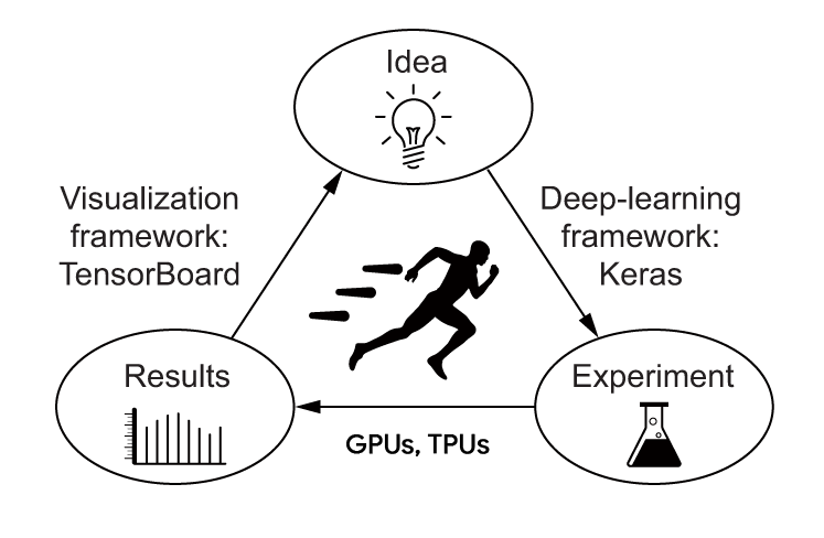
As you develop your expertise in the Keras API, how fast you can code up your deep learning experiments will cease to be the bottleneck of this progress cycle. The next bottleneck will become the speed at which you can train your models. Fast training infrastructure means that you can get your results back in 10 or 15 minutes and, hence, that you can go through dozens of iterations every day. Faster training directly improves the quality of your deep learning solutions.

In this section, you’ll learn about how to scale up your training runs by using multiple GPUs or TPUs.

18.2.1 Multi-GPU training

Although GPUs are becoming more powerful each year, deep learning models are also growing larger, requiring ever more computational resources. Training on a single GPU puts a hard bound on how fast you can move. The solution? We can simply add more GPUs and start doing multi-GPU distributed training.

There are two ways to distribute computation across multiple devices: data parallelism and model parallelism.

With data parallelism, a single model is replicated on multiple devices or multiple machines. Each model replica processes different batches of data, and then they merge their results.

With model parallelism, different parts of a single model run on different devices, processing a single batch of data together, at the same time. This works best with models that have a naturally parallel architecture, such as models that feature multiple branches. In practice, model parallelism is used only in the case of models that are too large to fit on any single device: it isn’t used as a way to speed up training of regular models, but as a way to train larger models.

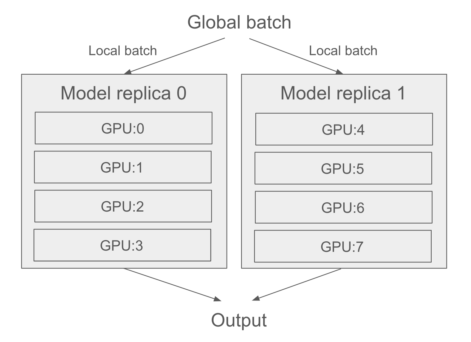
Then, of course, we can also mix both data parallelism and model parallelism: a single model can be split across multiple devices (e.g., 4), and that split model can be replicated across multiple groups of devices (e.g., twice, for a total of 2 * 4 = 8 devices used). Let’s see how this works in detail.

18.2.1.1 Data parallelism: Replicating a model on each GPU

Data parallelism is the most common form of distributed training. It operates on a simple principle: divide and conquer. Each GPU receives a copy of the entire model, called a replica. Incoming batches of data are split into N sub-batches, which are processed by one model replica each, in parallel. This is why it’s called data parallelism: different samples (data points) are processed in parallel. For instance, with two GPUs, a batch of size 128 is split into two sub-batches of size 64, which are processed by two model replicas. Then

In inference, we retrieve the predictions for each sub-batch and concatenate them to obtain the predictions for the full batch.
In training, we retrieve the gradients for each sub-batch, average them, and update all model replicas based on the gradient average. The state of the model is then the same as if we had trained it on the full batch of 128 samples. This is called synchronous training, because all replicas are kept in sync—their weights have the same value at all times. Nonsynchronous alternatives exist, but they are less efficient and are no longer used in practice.

Data parallelism is a simple and highly scalable way to train models faster. If you get more devices, just increase your batch size, and your training throughput increases accordingly. It has one limitation, though: it requires your model to be able to fit into one of your devices. However, it is now common to train foundation models that have tens of billions of parameters, which wouldn’t fit on any single GPU.

18.2.1.2 Model parallelism: Splitting our model across multiple GPUs

That’s where model parallelism comes in. Whereas data parallelism works by splitting batches of data into sub-batches and processing the sub-batches in parallel, model parallelism works by splitting the model into submodels and running each one on a different device—in parallel. For instance, consider the following model.

Listing 18.4: A large, densely connected model

model <- keras_model_sequential(input_shape = c(16000)) |>
  layer_dense(64000, activation = "relu") |>
  layer_dense(8000, activation = "sigmoid")

Each sample has 16,000 features and is classified into 8,000 potentially overlapping categories by two Dense layers. Those are large layers: the first has about 1 billion parameters, and the last has about 512 million parameters. If you’re working with two small devices, you won’t be able to use data parallelism because you can’t fit the model on a single device. What you can do is split a single instance of the model across multiple devices. This is often called “sharding” or “partitioning” a model. There are two main ways to split a model across devices: horizontal partitioning and vertical partitioning.

In horizontal partitioning, each device processes different layers of the model. For example, in the previous model, one GPU would handle the first Dense layer, and the other would handle the second Dense layer. The main drawback of this approach is that it can introduce communication overhead. For example, the output of the first layer needs to be copied to the second device before it can be processed by the second layer. This can become a bottleneck, especially if the output of the first layer is large—you’d risk keeping your GPUs idle.

In vertical partitioning, each layer is split across all available devices. Because layers are usually implemented in terms of matmul or convolution operations, which are highly parallelizable, this strategy is easy to implement in practice and is almost always the best fit for large models. For example, in the previous model, we could split the kernel and bias of the first Dense layer into two halves, so that each device only receives a kernel of shape (16000, 32000) (split along its last axis) and a bias of shape (32000). We’d compute op_matmul(inputs, kernel) + bias with this half-kernel and half-bias for each device and merge the two outputs by concatenating them like this:

.[half_kernel_0, half_kernel_1] <- op_split(kernel, 2)
.[half_bias_0, half_bias_1] <- op_split(bias, 2)

with(keras$device("gpu:0"), {
  half_output_0 <- op_matmul(inputs, half_kernel_0) + half_bias_0
})

with(keras$device("gpu:1"), {
  half_output_1 <- op_matmul(inputs, half_kernel_1) + half_bias_1
})

In reality, you will want to mix data parallelism and model parallelism. You will split your model across, say, four devices, and you will replicate that split model across multiple groups of two devices—let’s say two—each processing one sub-batch of data in parallel. You will then have two replicas, each running on four devices, for a total of eight devices used (figure 18.2).

Distributing a model across eight devices: two model replicas, each handled by a group of 4 devices

18.2.2 Distributed training in practice

Now let’s see how to implement these concepts in practice. We will only cover the JAX backend, as it is the most performant and most scalable of the various Keras backends by a mile. If you’re doing any kind of large-scale distributed training and you aren’t using JAX, you’re making a mistake—and wasting dollars burning much more compute than you actually need.

18.2.2.1 Getting your hands on two or more GPUs

First, you need to get access to several GPUs. As of now, Google Colab lets you use only a single GPU, so you will need to do one of two things:

Acquire two to eight GPUs, mount them on a single machine (it will require a beefy power supply), and install CUDA drivers, cuDNN, etc. For most people, this isn’t the best option.
Rent a multi-GPU virtual machine (VM) on Google Cloud, Azure, or AWS. You’ll be able to use VM images with preinstalled drivers and software, and you’ll have very little setup overhead. This is likely the best option for anyone who isn’t training models 24/7.

We won’t cover the details of how to spin up multi-GPU cloud VMs because such instructions would be relatively short-lived, and this information is readily available online.

18.2.2.2 Using data parallelism with JAX

Using data parallelism with Keras and JAX is very simple: before building our model, we add the following line of code:

keras$distribution$set_distribution(
  keras$distribution$DataParallel()
)

That’s it. If you want more granular control, you can specify which devices you want to use. You can list available devices via

keras$distribution$list_devices()

[1] "gpu:0" "gpu:1"

It will return a list of strings—the names of your devices, such as "gpu:0", "gpu:1", and so on. You can then pass these to the DataParallel constructor:

keras$distribution$set_distribution(
  keras$distribution$DataParallel(devices = c("gpu:0", "gpu:1"))
)

In an ideal world, training on N GPUs would result in a speedup of factor N. In practice, however, distribution introduces some overhead—in particular, merging the weight deltas originating from different devices takes some time. The effective speedup you get is a function of the number of GPUs used:

With two GPUs, the speedup stays close to 2×.
With four, the speedup is around 3.8×.
With eight, it’s around 7.3×.

This assumes that you’re using a large enough global batch size to keep each GPU utilized at full capacity. If your batch size is too small, the local batch size won’t be enough to keep your GPUs busy.

18.2.2.3 Using model parallelism with JAX

Keras also provides powerful tools for fully customizing how we want to do distributed training, including model parallel training and any mixture of data parallel and model parallel training you can imagine. Let’s dive in.

18.2.2.3.1 The DeviceMesh API

First, you need to understand the concept of device mesh. A device mesh is simply a grid of devices. Consider this example, with eight GPUs:

gpu:0   |   gpu:4
--------|---------
gpu:1   |   gpu:5
--------|---------
gpu:2   |   gpu:6
--------|---------
gpu:3   |   gpu:7

The big idea is to separate devices into groups, organized along axes. Typically, one axis will be responsible for data parallelism, and one axis will be responsible for model parallelism (as in figure 18.2, your devices form a grid, where the horizontal axis handles data parallelism and the vertical axis handles model parallelism).

A device mesh doesn’t have to be 2D—it could be any shape you want. In practice, however, you will only ever see 1D and 2D meshes.

Let’s make a 2 × 4 device mesh in Keras:

device_mesh <- keras$distribution$DeviceMesh(
1  shape = shape(2, 4),
2  axis_names = c("data", "model")
)

1: We assume 8 devices, organized as a 2 × 4 grid
2: It’s convenient to give the axes meaningful names!

Mind you, you can also explicitly specify the devices you want to use:

devices <- paste0("gpu:", 0:7)
device_mesh <- keras$distribution$DeviceMesh(
  shape = shape(2, 4),
  axis_names = c("data", "model"),
  devices = devices
)

As you may have guessed from the axis_names argument, we intend to use the devices along the first axis for data parallelism and the devices along axis 1 for model parallelism. Because there are two devices along the first axis and four along the second axis, we’ll split our model’s computation across four GPUs, and we’ll make two copies of our split model, running each copy on a different sub-batch of data in parallel.

Now that we have our mesh, we need to tell Keras how to split different pieces of computation across our devices. For that, we’ll use the LayoutMap API.

18.2.2.3.2 The LayoutMap API

To specify where different bits of computation should take place, we use variables as our frame of reference. We will split or replicate variables across our devices, and we will let the compiler move all computation associated with that part of the variable to the corresponding device.

Consider a variable. Its shape is, let’s say, (32, 64). There are two things we can do with this variable:

Replicate it (copy it) across an axis of our mesh, so each device along that axis sees the same value.
Shard it (split it) across an axis of our mesh—for instance, into four chunks of shape (32, 16)—so that each device along that axis sees one different chunk.

Note that our variable has two dimensions. Importantly, we can make “sharding” or “replicating” decisions independently for each dimension of the variable.

The API we use to tell Keras about such decisions is the LayoutMap class. A LayoutMap is similar to a dictionary. It maps model variables (for instance, the kernel variable of the first Dense layer in our model) to a bit of information about how that variable should be replicated or sharded over a device mesh. Specifically, it maps a variable path to a tuple that has as many entries as our variable has dimensions, where each entry specifies what to do with that variable dimension. It looks like this:

list(
1  "sequential/dense_1/kernel" = tuple(NULL, "model"),
2  "sequential/dense_1/bias" = tuple("model"),
  ...
)

1: NULL means “replicate the variable along this dimension.”
2: "model" means “shard the variable along this dimension across the devices of the ‘model’ axis of the device mesh.”

If this is the first time you’ve encountered the concept of a variable path, it is simply a string identifier that looks like "sequential/dense_1/kernel". It’s a useful way to refer to a variable without keeping a handle on the actual variable instance.

Here’s how to print the paths for all variables in a model:

for (v in model$variables)
  cat(v$path, "\n")

sequential_1/dense_2/kernel 
sequential_1/dense_2/bias 
sequential_1/dense_3/kernel 
sequential_1/dense_3/bias

Now let’s shard and replicate these variables. In the case of a simple model like this one, our go-to rule of thumb for variable sharding is as follows:

Shard the last dimension of the variable along the "model" mesh axis.
Leave all other dimensions as replicated.

Simple enough, right? Like this:

layout_map <- keras$distribution$LayoutMap(device_mesh)
layout_map["sequential/dense/kernel"]   <- tuple(NULL, "model")
layout_map["sequential/dense/bias"]     <- tuple("model")
layout_map["sequential/dense_1/kernel"] <- tuple(NULL, "model")
layout_map["sequential/dense_1/bias"]   <- tuple("model")

Finally, we tell Keras to refer to this sharding layout when instantiating the variables by setting the distribution configuration like this:

model_parallel <- keras$distribution$ModelParallel(
  layout_map = layout_map,
1  batch_dim_name = "data"
)
keras$distribution$set_distribution(model_parallel)

1: Tells Keras to use the mesh axis named “data” for data parallelism

Once the distribution configuration is set, you can create your model and fit() it. No other part of your code changes—the model definition code is the same, and the training code is the same. That’s true whether you’re using built-in APIs like fit() and evaluate() or your own training logic. Assuming that you have the right LayoutMap for your variables, the little code snippets you just saw are enough to distribute computation for any large language model training run—it scales to as many devices as you have available and arbitrary model sizes.

To check how our variables were sharded, we can inspect the variable$value$sharding property, like this:

model$layers[[1]]$kernel$value$sharding

SingleDeviceSharding(device=CudaDevice(id=0), memory_kind=device)

We can even visualize it via the JAX utility jax$debug$visualize_sharding:

jax <- reticulate::import("jax")
value <- model$layers[[1]]$kernel$value
jax$debug$visualize_sharding(value$shape, value$sharding)

Tip

When doing distributed training, always provide your data as a tf.data.Dataset object to guarantee best performance (passing your data as R or NumPy arrays also works because those are converted to Dataset objects by fit()). You should also be sure to use data prefetching: before passing the dataset to fit(), call dataset_prefetch(buffer_size). If you aren’t sure what buffer size to pick, leave the default value dataset_prefetch(buffer_size = tf$data$AUTOTUNE) option, which will pick a buffer size for you.

18.2.3 TPU training

Beyond GPUs, there is generally a trend in the deep learning world toward moving workflows to increasingly specialized hardware designed specifically for deep learning workflows. Such single-purpose chips are known as application-specific integrated circuits (ASICs). Various companies, big and small, are working on new chips, but today the most prominent effort along these lines is Google’s tensor processing unit (TPU), which is available on Google Cloud and via Google Colab.

Training on TPU does involve jumping through some hoops. But it’s worth the extra work: TPUs are really, really fast. Training on a TPU V2 (available on Colab) will typically be 15× faster than training on an NVIDIA P100 GPU. For most models, TPU training ends up being 3× more cost-effective than GPU training on average.

You can actually use TPU v2 for free in Colab. In the Colab menu, under the Runtime tab, in the Change Runtime Type option, you’ll notice that you have access to a TPU runtime in addition to the GPU runtime. For more serious training runs, Google Cloud also makes available TPU v3 through v5, which are even faster.

When running Keras code with the JAX backend on a TPU-enabled notebook, you don’t need anything more than calling keras$distribution$set_distribution(distribution) with a DataParallel or ModelParallel distribution instance to start using TPU cores. Be sure to call it before creating your model!

Tip

Because TPUs can process batches of data extremely quickly, the speed at which you can read data from Google Cloud Storage (GCS) can easily become a bottleneck. If your dataset is small enough, you should keep it in the memory of the VM. You can do so by calling dataset_cache() on your tf.data.Dataset instance. That way, the data will be read from GCS only once.

18.2.3.1 Using step fusing to improve TPU utilization

Because a TPU has a lot of compute power available, you need to train with very large batches to keep the TPU cores busy. For small models, the batch size required can be extraordinarily large—upward of 10,000 samples per batch. When working with enormous batches, you should be sure to increase your optimizer learning rate accordingly: you’re going to be making fewer updates to your weights, but each update will be more accurate (because the gradients are computed using more data points); hence, you should move the weights by a greater magnitude with each update.

There is, however, a simple trick you can use to keep reasonably sized batches while maintaining full TPU utilization: step fusing. The idea is to run multiple steps of training during each TPU execution step. Basically, do more work in between two round-trips from the VM memory to the TPU. To do this, simply specify the steps_per_execution argument in compile(): for instance, steps_per_execution=8 to run eight steps of training during each TPU execution. For small models that are underutilizing the TPU, this can result in a dramatic speedup:

model |> compile(..., steps_per_execution = 8)

18.3 Speeding up training and inference with lower-precision computation

View on GitHub Run on Colab

What if we told you there’s a simple technique you can use to speed up training and inference of almost any model by up to 2×, basically for free? It seems too good to be true, and yet such a trick does exist. To understand how it works, first we need to take a look at the notion of “precision” in computer science.

18.3.1 Understanding floating-point precision

Precision is to numbers what resolution is to images. Because computers can only process 1s and 0s, any number seen by a computer has to be encoded as a binary string. For instance, you may be familiar with uint8 integers, which are integers encoded on eight bits: 00000000 represents 0 in uint8, and 11111111 represents 255. To represent integers beyond 255, you need to add more bits—eight isn’t enough. Most integers are stored on 32 bits, which can represent signed integers ranging from -2,147,483,648 to 2,147,483,647.

Floating-point numbers are the same. In mathematics, real numbers form a continuous axis: there are an infinite number of points in between any two numbers. We can always zoom in on the axis of reals. In computer science, this isn’t true: there’s a finite number of intermediate points between 3 and 4, for instance. How many? Well, it depends on the precision we’re working with: the number of bits we’re using to store a number. We can only zoom up to a certain resolution.

There are three levels of precision we typically use:

Half precision, or float16, where numbers are stored on 16 bits
Single precision, or float32, where numbers are stored on 32 bits
Double precision, or float64, where numbers are stored on 64 bits

We can even go down to float8, as you’ll see in a bit.

On floating-point encoding

A counterintuitive fact about floating-point numbers is that representable numbers are not uniformly distributed. Larger numbers have lower precision: there are the same number of representable values between 2^N and 2^(N+1) as between 1 and 2, for any N.

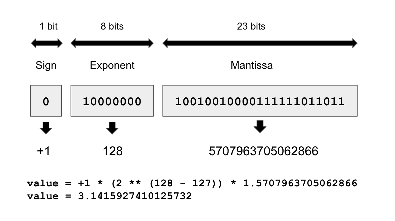
That’s because floating-point numbers are encoded in three parts: the sign, the significant value (called the mantissa), and the exponent, in the form

{sign} * (2 ^ ({exponent} - 127)) * 1.{mantissa}

For example, the following diagram demonstrates how to encode the closest float32 value approximating pi.

The number pi encoded in single precision via a sign bit, an integer exponent, and an integer mantissa.

For this reason, the numerical error incurred when converting a number to its floating-point representation can vary wildly depending on the exact value considered, and the error tends to get larger for numbers with a large absolute value.

The way to think about the resolution of floating-point numbers is in terms of the smallest distance between two arbitrary numbers that you’ll be able to safely process. In single precision, that’s around 1e-7. In double precision, that’s around 1e-16. And in half precision, it’s only 1e-3.

18.3.2 Float16 inference

Every model you’ve seen in this book so far has used single-precision numbers: it stored its state as float32 weight variables and ran its computations on float32 inputs. That’s enough precision to run the forward and backward passes of a model without losing any information—in particular when it comes to small gradient updates (recall that the typical learning rate is 1e-3, and it’s pretty common to see weight updates on the order of 1e-6).

Modern GPUs and TPUs feature specialized hardware that can run 16-bit operations much more quickly and use less memory than equivalent 32-bit operations. By using these lower-precision operations whenever possible, you can speed up training on those devices by a significant factor. You can set the default floating-point precision to float16 in Keras via

config_set_dtype_policy("float16")

Note that this should be done before you define your model. Doing this will net you a nice speedup for model inference, for instance, via model |> predict(). You should expect a nearly 2× speed boost on GPU and TPU.

There’s also an alternative to float16 that works better on some devices, in particular TPUs: bfloat16. bfloat16 is also a 16-bit precision floating-point type, but it differs from float16 in its structure: it uses 8 exponent bits instead of 5, and 7 mantissa bits instead of 10 (see table 18.1). This means it can cover a much wider range of values, but it has a lower “resolution” over this range. Some devices are better optimized for bfloat16 compared to float16, so it can be a good idea to try both before settling for the option that turns out to be the fastest.

Difference between `float16` and `bfloat16`
dtype	float16	bfloat16
Exponent bits	5	8
Mantissa bits	10	7
Sign bits	1	1

18.3.3 Mixed-precision training

Setting your default float precision to 16 bits is a great way to speed up inference. But when it comes to training, there’s a significant complication. The gradient descent process won’t run smoothly in float16 or bfloat16, because you can’t represent small gradient updates of around 1e-5 or 1e-6, which are common.

You can, however, use a hybrid approach: that’s what mixed-precision training is about. The idea is to use 16-bit computation in places where precision isn’t a problem, while working with 32-bit values in other places to maintain numerical stability—in particular, when handling gradients and variable updates. By maintaining the precision-sensitive parts of the model in full precision, you can get most of the speed benefits of 16-bit computation without meaningfully affecting model quality.

You can turn on mixed precision like this:

config_set_dtype_policy("mixed_float16")

Typically, most of the forward pass of the model will be done in float16 (with the exception of numerically unstable operations like softmax), but the weights of the model will be stored and updated in float32. Your float16 gradients will be cast to float32 before updating the float32 variables.

Keras layers have a variable_dtype and a compute_dtype attribute. By default, both of these are set to float32. When we turn on mixed precision, the compute_dtype of most layers switches to float16. As a result, those layers will cast their inputs to float16 and will perform their computation in float16 (using half-precision copies of the weights). However, because their variable_dtype is still float32, their weights will be able to receive accurate float32 updates from the optimizer, as opposed to half-precision updates.

Some operations may be numerically unstable in float16 (in particular, softmax and cross-entropy). If you need to opt out of mixed precision for a specific layer, just pass the argument dtype="float32" to the constructor of this layer.

18.3.4 Using loss scaling with mixed precision

During training, gradients can become very small. When using mixed precision, our gradients remain in float16 (same as the forward pass). As a result, the limited range of representable numbers can cause small gradients to be rounded down to zero. This prevents the model from learning effectively.

Gradient values are proportional to the loss value, so to encourage gradients to be larger, a simple trick is to multiply the loss by a large scalar factor. Your gradients will then be much less likely to get rounded to zero.

Keras makes this easy. If you want to use a fixed loss scaling factor, you can simply pass a loss_scale_factor argument to your optimizer like this:

optimizer <- optimizer_adam(learning_rate = 1e-3, loss_scale_factor = 10)

If you would like the optimizer to automatically figure out the right scaling factor, you can also use the LossScaleOptimizer wrapper:

optimizer <-
  optimizer_adam(learning_rate = 1e-3) |>
  optimizer_loss_scale()

Using LossScaleOptimizer is usually your best option: the right scaling value can change over the course of training!

18.3.5 Beyond mixed precision: float8 training

If running a forward pass in 16-bit precision yields such neat performance benefits, you may wonder, could we go even lower? What about 8-bit precision? Four bits, maybe? Two bits? The answer is, it’s complicated.

Mixed-precision training using float16 in the forward pass is that last level of precision that “just works”: float16 precision has enough bits to represent all intermediate tensors (except for gradient updates, which is why we use float32 for those). This is no longer true if you go down to float8 precision: you are simply losing too much information. It is still possible to use float8 in some computations, but this requires you to make considerable modifications to your forward pass. You will not be able to simply set your compute_dtype to float8 and run.

The Keras framework provides a built-in implementation for float8 training. Because it specifically targets Transformer use cases, it only covers a restricted set of layers: Dense, EinsumDense (the version of Dense that is used by the MultiHeadAttention layer), and Embedding layers. The way it works is not simple: it keeps track of past activation values to rescale activations at each step so as to utilize the full range of values representable in float8. It also needs to override part of the backward pass to do the same with gradient values.

Importantly, this added overhead has a computational cost. If your model is too small or if your GPU isn’t powerful enough, that cost will exceed the benefits of doing certain operations in float8, and you will see a slowdown instead of a speedup. float8 training is only viable for very large models (typically over 5 billion parameters) and large, recent GPUs such as the NVIDIA H100. float8 is rarely used in practice, except in foundation model training runs.

18.3.6 Faster inference with quantization

Running inference in float16—or even float8—will result in a nice speedup for your models. But there’s also another trick you can use: int8 quantization. The big idea is to take an already trained model with weights in float32, and convert these weights to a lower-precision dtype (typically int8) while preserving the numerical correctness of the forward pass as much as possible.

If you want to implement quantization from scratch, the math is simple: the general idea is to scale all matmul input tensors by a certain factor so that their coefficients fit in the range representable with int8, which is [-127, 127]: a total of 256 possible values. After scaling the inputs, you cast them to int8 and perform the matmul operation in int8 precision, which should be quite a bit faster than float16. Finally, you cast the output back to float32, and you divide it by the product of the input scaling factors. Because matmul is a linear operation, this final unscaling cancels out the initial scaling, and you should get the same output as if you used the original values—any loss of accuracy only comes from the value rounding that happens when you cast the inputs to int8.

Let’s make this concrete with an example. Let’s say we want to perform matmul(x, kernel), with the following values:

x <- op_array(rbind(c(0.1, 0.9), c(1.2, -0.8)))
kernel <- op_array(rbind(c(-0.1, -2.2), c(1.1, 0.7)))

If we were to naively cast these values to int8 without scaling first, that would be very destructive—for instance, our x would become [[0, 0], [1, 0]]. So let’s apply the “abs-max” scaling scheme, which spreads out the values of each tensor across the [-127, 127] range:

abs_max_quantize <- function(value) {
1  abs_max <- op_max(op_abs(value), keepdims = TRUE)
2  scale <- op_divide(127, abs_max + 1e-7)
3  scaled_value <- value * scale
4  scaled_value <- op_clip(op_round(scaled_value), -127, 127)
5  scaled_value <- op_cast(scaled_value, dtype = "int8")
  list(scaled_value, scale)
}

.[int_x, x_scale] <- abs_max_quantize(x)
.[int_kernel, kernel_scale] <- abs_max_quantize(kernel)

1: Max of the absolute value of the tensor
2: Scale is the max of the int range divided by the max of the tensor (1e-7 is to avoid dividing by 0).
3: Scales the value
4: Rounding and clipping first is more accurate than directly casting.
5: Casts to int8

Now we can perform a faster matmul and unscale the output:

int_y <- op_matmul(int_x, int_kernel)
y <- op_cast(int_y, dtype = "float32") / (x_scale * kernel_scale)

How accurate is it? Let’s compare our y with the output of the float32 matmul:

Array([[ 0.9843737 ,  0.39332393],
       [-1.0151457 , -3.196514  ]], dtype=float32)

op_matmul(x, kernel)

Array([[ 0.98      ,  0.40999997],
       [-1.        , -3.2       ]], dtype=float32)

Pretty accurate! For a large matmul, doing this will save you a lot of compute. int8 computation can be considerably faster than even float16 computation, and you only have to add fairly fast elementwise ops to the computation graphs: abs, max, clip, cast, divide, multiply.

Of course, we don’t expect you to ever implement quantization by hand—that would be tremendously impractical. Similar to float8, int8 quantization is built directly into specific Keras layers: Dense, EinsumDense, and Embedding. This unlocks int8 inference support for any Transformer-based model. Here’s how to use it with any Keras model that includes such layers:

1model <- ...
2model |> quantize_weights("int8")
3predictions <- model |> predict(...)

1: Instantiates a model (or any quantizable layer)
2: Boom!
3: Now, predict() and call() will run (partially) in int8!

18.4 Summary

You can use hyperparameter tuning and KerasTuner to automate the tedium out of finding the best model configuration. But be mindful of validation-set overfitting!
An ensemble of diverse models can often significantly improve the quality of your predictions.
To further scale your workflows, you can use data parallelism to train a model on multiple devices, as long as the model is small enough to fit on a single device.
For larger models, you can also use model parallelism to split your model’s variables and computation across several devices.
You can speed up model training on GPU or TPU by turning on mixed precision—you’ll generally get a nice speed boost at virtually no cost.
You can also speed up inference by using float16 precision or even int8 quantization.