

Sequential class
library(keras3)

model <- keras_model_sequential() |>
  layer_dense(64, activation = "relu") |>
layer_dense(10, activation = "softmax")This chapter covers
Sequential class, the Functional API, and model subclassingYou’re starting to have some experience with Keras. You’re familiar with the Sequential model, Dense layers, and built-in APIs for training, evaluation, and inference: compile(), fit(), evaluate(), and predict(). You even learned in chapter 3 how to inherit from the Layer class to create custom layers, and how to use the gradient APIs in TensorFlow, JAX, and PyTorch to implement a step-by-step training loop.
In the coming chapters, we’ll dig into computer vision, timeseries forecasting, natural language processing, and generative deep learning. These complex applications will require much more than a Sequential architecture and the default fit() loop. So let’s first turn you into a Keras expert! In this chapter, you’ll get a complete overview of the key ways to work with Keras APIs: everything you’re going to need to handle the advanced deep learning use cases you’ll encounter next.
The design of the Keras API is guided by the principle of progressive disclosure of complexity: make it easy to get started, yet make it possible to handle high-complexity use cases while requiring only incremental learning at each step. Simple use cases should be easy and approachable, and arbitrarily advanced workflows should be possible: no matter how niche and complex the thing we want to do, there should be a clear path to it: a path that builds on things learned from simpler workflows. This means you can grow from beginner to expert and still use the same tools—only in different ways.
As such, there’s not a single “true” way to use Keras. Rather, Keras offers a spectrum of workflows, from the very simple to the very flexible. There are different ways to build Keras models and different ways to train them, answering different needs.
For instance, we have a range of ways to build models and an array of ways to train them, each representing a certain tradeoff between usability and flexibility. We can use Keras as we would use tidymodels—just calling fit() and letting the framework do its thing—or we can use it like base R—taking full control of every little detail.
Because all these workflows are based on shared APIs, such as Layer and Model, components from any workflow can be used in any other workflow: they can all talk to each other. This means everything you’re learning will still be relevant once you’ve become an expert. You can get started easily and then gradually dive into workflows where you’re writing more logic from scratch. You won’t have to switch to an entirely different framework as you go from student to researcher, or from data scientist to deep learning engineer.
This philosophy is not unlike that of R itself! Some languages offer only one way to write programs: for instance, object-oriented programming or functional programming. Meanwhile, R is a multi-paradigm language: it offers a range of possible usage patterns, which all work nicely together. This makes R suitable for a wide range of different use cases. Likewise, you can think of Keras as the R of deep learning: a user-friendly deep learning language that offers a variety of workflows for different user profiles.
There are three APIs for building models in Keras, as shown in figure 7.1:
Sequential model—The most approachable API; it’s basically a flat list. As such, it’s limited to simple stacks of layers.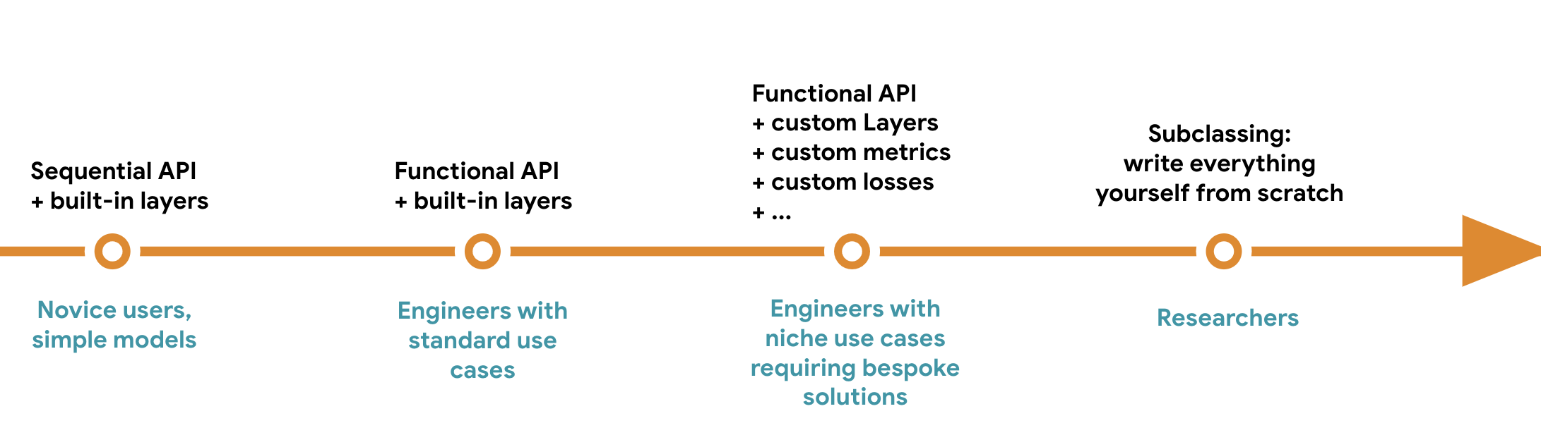
The simplest way to build a Keras model is using the Sequential model with keras_model_sequential(), which you already know about.
Sequential class
library(keras3)
model <- keras_model_sequential() |>
layer_dense(64, activation = "relu") |>
layer_dense(10, activation = "softmax")Note that it’s possible to build the same model incrementally, by passing it to a layer constructor. This appends a layer to the model’s layers list.
Sequential model
model <- keras_model_sequential()
model |> layer_dense(64, activation = "relu")
model |> layer_dense(10, activation = "softmax")
You saw in chapter 3 that layers only get built (which is to say, their weights are created) when they are called for the first time. That’s because the shape of the layers’ weights depends on the shape of their input: until the input shape is known, they can’t be created. As such, the previous Sequential model does not have any weights until we call it on some data or call its build() method with an input shape.
1model$weightslist()NA in the input shape signals that the batch size could be anything.
List of 4
 $ :<Variable path=sequential_1/dense_2/kernel, shape=(3, 64), dtype=float32, value=[…]>
 $ :<Variable path=sequential_1/dense_2/bias, shape=(64), dtype=float32, value=[…]>
 $ :<Variable path=sequential_1/dense_3/kernel, shape=(64, 10), dtype=float32, value=[…]>
 $ :<Variable path=sequential_1/dense_3/bias, shape=(10), dtype=float32, value=[…]>
After the model is built, we can display its contents via the print() method, which comes in handy for debugging.
modelModel: "sequential_1"
┏━━━━━━━━━━━━━━━━━━━━━━━━━━━━━━━━━┳━━━━━━━━━━━━━━━━━━━━━━━━┳━━━━━━━━━━━━━━━┓
┃ Layer (type) ┃ Output Shape ┃ Param # ┃
┡━━━━━━━━━━━━━━━━━━━━━━━━━━━━━━━━━╇━━━━━━━━━━━━━━━━━━━━━━━━╇━━━━━━━━━━━━━━━┩
│ dense_2 (Dense) │ (None, 64) │ 256 │
├─────────────────────────────────┼────────────────────────┼───────────────┤
│ dense_3 (Dense) │ (None, 10) │ 650 │
└─────────────────────────────────┴────────────────────────┴───────────────┘
Total params: 906 (3.54 KB)
Trainable params: 906 (3.54 KB)
Non-trainable params: 0 (0.00 B)
As you can see, this model happens to be named “sequential_1”. We can give names to everything in Keras—every model and every layer.
name argument
model <- keras_model_sequential(name = "my_example_model")
model |> layer_dense(64, activation = "relu", name = "my_first_layer")
model |> layer_dense(10, activation = "softmax", name = "my_last_layer")
model$build(shape(NA, 3))
model
Model: "my_example_model"
┏━━━━━━━━━━━━━━━━━━━━━━━━━━━━━━━━━┳━━━━━━━━━━━━━━━━━━━━━━━━┳━━━━━━━━━━━━━━━┓
┃ Layer (type) ┃ Output Shape ┃ Param # ┃
┡━━━━━━━━━━━━━━━━━━━━━━━━━━━━━━━━━╇━━━━━━━━━━━━━━━━━━━━━━━━╇━━━━━━━━━━━━━━━┩
│ my_first_layer (Dense) │ (None, 64) │ 256 │
├─────────────────────────────────┼────────────────────────┼───────────────┤
│ my_last_layer (Dense) │ (None, 10) │ 650 │
└─────────────────────────────────┴────────────────────────┴───────────────┘
Total params: 906 (3.54 KB)
Trainable params: 906 (3.54 KB)
Non-trainable params: 0 (0.00 B)
When building a Sequential model incrementally, it’s useful to be able to print a summary of what the current model looks like after we add each layer. But we can’t print a summary until the model is built! There’s a way to have a Sequential model be built on the fly: declare the shape of the model’s inputs in advance. We can do this via the input_shape argument.
1model <- keras_model_sequential(input_shape = c(3))
model |> layer_dense(64, activation = "relu")Now we can use print() to follow how the output shape of the model changes as we add more layers:
modelModel: "sequential_2"
┏━━━━━━━━━━━━━━━━━━━━━━━━━━━━━━━━━┳━━━━━━━━━━━━━━━━━━━━━━━━┳━━━━━━━━━━━━━━━┓
┃ Layer (type) ┃ Output Shape ┃ Param # ┃
┡━━━━━━━━━━━━━━━━━━━━━━━━━━━━━━━━━╇━━━━━━━━━━━━━━━━━━━━━━━━╇━━━━━━━━━━━━━━━┩
│ dense_4 (Dense) │ (None, 64) │ 256 │
└─────────────────────────────────┴────────────────────────┴───────────────┘
Total params: 256 (1.00 KB)
Trainable params: 256 (1.00 KB)
Non-trainable params: 0 (0.00 B)
model |> layer_dense(10, activation = "softmax")
model
Model: "sequential_2"
┏━━━━━━━━━━━━━━━━━━━━━━━━━━━━━━━━━┳━━━━━━━━━━━━━━━━━━━━━━━━┳━━━━━━━━━━━━━━━┓
┃ Layer (type) ┃ Output Shape ┃ Param # ┃
┡━━━━━━━━━━━━━━━━━━━━━━━━━━━━━━━━━╇━━━━━━━━━━━━━━━━━━━━━━━━╇━━━━━━━━━━━━━━━┩
│ dense_4 (Dense) │ (None, 64) │ 256 │
├─────────────────────────────────┼────────────────────────┼───────────────┤
│ dense_5 (Dense) │ (None, 10) │ 650 │
└─────────────────────────────────┴────────────────────────┴───────────────┘
Total params: 906 (3.54 KB)
Trainable params: 906 (3.54 KB)
Non-trainable params: 0 (0.00 B)
This is a pretty common debugging workflow when dealing with layers that transform their inputs in complex ways, such as the convolutional layers you’ll learn about in chapter 8.
The Sequential model is easy to use, but its applicability is extremely limited: it can only express models with a single input and a single output, applying one layer after the other in a sequential fashion. In practice, it’s common to encounter models with multiple inputs (say, an image and its metadata), multiple outputs (different things we want to predict about the data), or a nonlinear topology.
In such cases, we build our model using the Functional API. This is what most Keras models you’ll encounter in the wild use. It’s fun and powerful—it feels like playing with LEGO bricks.
Let’s start with something simple: the two-layer stack we used in the previous section. Its Functional API version looks like the following listing.
Dense layers
inputs <- keras_input(shape = c(3), name = "my_input")
features <- inputs |> layer_dense(64, activation = "relu")
outputs <- features |> layer_dense(10, activation = "softmax")
model <- keras_model(inputs = inputs, outputs = outputs,
                     name = "my_functional_model")
Let’s go over this step by step. We start by creating a keras_input() (note that you can also give names to these input objects, like everything else):
inputs <- keras_input(shape = c(3), name = "my_input")This inputs object holds information about the shape and dtype of the data the model will process:
1op_shape(inputs)shape(NA, 3)We call such an object a symbolic tensor. It doesn’t contain any actual data, but it encodes the specifications of the actual tensors of data that the model will see when we use it. It stands for future tensors of data.
Next, we create a layer and call it on the input:
features <- inputs |> layer_dense(64, activation = "relu")All Keras layers can be called on real tensors of data or on these symbolic tensors. In the latter case, they return a new symbolic tensor, with updated shape and dtype information:
op_shape(features)shape(NA, 64)After obtaining the final outputs, we instantiate the model by specifying its inputs and outputs in the Model constructor:
outputs <- features |> layer_dense(10, activation = "softmax")
model <- keras_model(inputs = inputs, outputs = outputs,
                     name = "my_functional_model")
Here’s the summary of our model:
modelModel: "my_functional_model"
┏━━━━━━━━━━━━━━━━━━━━━━━━━━━━━━━━━┳━━━━━━━━━━━━━━━━━━━━━━━━┳━━━━━━━━━━━━━━━┓
┃ Layer (type) ┃ Output Shape ┃ Param # ┃
┡━━━━━━━━━━━━━━━━━━━━━━━━━━━━━━━━━╇━━━━━━━━━━━━━━━━━━━━━━━━╇━━━━━━━━━━━━━━━┩
│ my_input (InputLayer) │ (None, 3) │ 0 │
├─────────────────────────────────┼────────────────────────┼───────────────┤
│ dense_8 (Dense) │ (None, 64) │ 256 │
├─────────────────────────────────┼────────────────────────┼───────────────┤
│ dense_9 (Dense) │ (None, 10) │ 650 │
└─────────────────────────────────┴────────────────────────┴───────────────┘
Total params: 906 (3.54 KB)
Trainable params: 906 (3.54 KB)
Non-trainable params: 0 (0.00 B)
Unlike this toy model, most deep learning models don’t look like lists—they look like graphs. They may, for instance, have multiple inputs or multiple outputs. It’s for this kind of model that the Functional API really shines.
Let’s say we’re building a system to rank customer support tickets by priority and route them to the appropriate department. Our model has three inputs:
We can encode the text inputs as arrays of ones and zeros of size vocabulary_size (see chapter 14 for detailed information about text encoding techniques).
The model also has two outputs:
We can build this model in a few lines with the Functional API. The Functional API is a simple, LEGO-like, yet very flexible way to define arbitrary graphs of layers like these.
vocabulary_size <- 10000
num_tags <- 100
num_departments <- 4

1title <- keras_input(c(vocabulary_size), name = "title")
text_body <- keras_input(c(vocabulary_size), name = "text_body")
tags <- keras_input(c(num_tags), name = "tags")

features <-
2  layer_concatenate(c(title, text_body, tags)) |>
3  layer_dense(64, activation = "relu", name = "dense_features")

4priority <- features |>
  layer_dense(1, activation = "sigmoid", name = "priority")

department <- features |>
  layer_dense(num_departments, activation = "softmax", name = "department")

5model <- keras_model(
  inputs = c(title, text_body, tags),
  outputs = c(priority, department)
)We can train our model in much the same way we would train a Sequential model: by calling fit() with lists of input and output data. These lists of data should respect the same order we passed to the Model constructor (keras_model()).
num_samples <- 1280

random_uniform_array <- function(dim) {
  array(runif(prod(dim)), dim)
}

random_integer_array <- function(dim, minval = 0L, maxval = 1L) {
  array(sample(minval:maxval, prod(dim), replace = TRUE), dim)
}

1title_data     <- random_integer_array(c(num_samples, vocabulary_size))
text_body_data <- random_integer_array(c(num_samples, vocabulary_size))
tags_data      <- random_integer_array(c(num_samples, num_tags))

2priority_data <- random_uniform_array(c(num_samples, 1))
department_data <- random_integer_array(
  dim = c(num_samples, 1),
  maxval = num_departments - 1
)

model |> compile(
  optimizer = "adam",
  loss = c("mean_squared_error", "sparse_categorical_crossentropy"),
  metrics = list(c("mean_absolute_error"), c("accuracy"))
)

model |> fit(
  x = list(title_data, text_body_data, tags_data),
  y = list(priority_data, department_data),
  epochs = 1
)

model |> evaluate(
  x = list(title_data, text_body_data, tags_data),
  y = list(priority_data, department_data)
)

.[priority_preds, department_preds] <- model |> predict(
  list(title_data, text_body_data, tags_data)
)If we don’t want to rely on input order (for instance, because we have many inputs or outputs), we can also use the names we gave the keras_input() objects and output layers, and pass data via named lists.
model |> compile(
  optimizer = "adam",
  loss = list(
    priority = "mean_squared_error",
    department = "sparse_categorical_crossentropy"
  ),
  metrics = list(
    priority = c("mean_absolute_error"),
    department = c("accuracy")
  )
)

model |> fit(
  x = list(title = title_data, text_body = text_body_data, tags = tags_data),
  y = list(priority = priority_data, department = department_data),
  epochs = 1
)

model |> evaluate(
  x = list(title = title_data, text_body = text_body_data, tags = tags_data),
  y = list(priority = priority_data, department = department_data)
)

.[priority_preds, department_preds] <- model |> predict(
  list(title = title_data, text_body = text_body_data, tags = tags_data)
)A Functional model is an explicit graph data structure. This makes it possible to inspect how layers are connected and reuse previous graph nodes (which are layer outputs) as part of new models. It also nicely fits the “mental model” that most researchers use when thinking about a deep neural network: a graph of layers.
This enables two important use cases: model visualization and feature extraction. Let’s take a look.
Let’s visualize the connectivity of the model we just defined (the topology of the model). We can plot a Functional model as a graph with the plot() method for models, as shown in figure 7.2:
plot(model)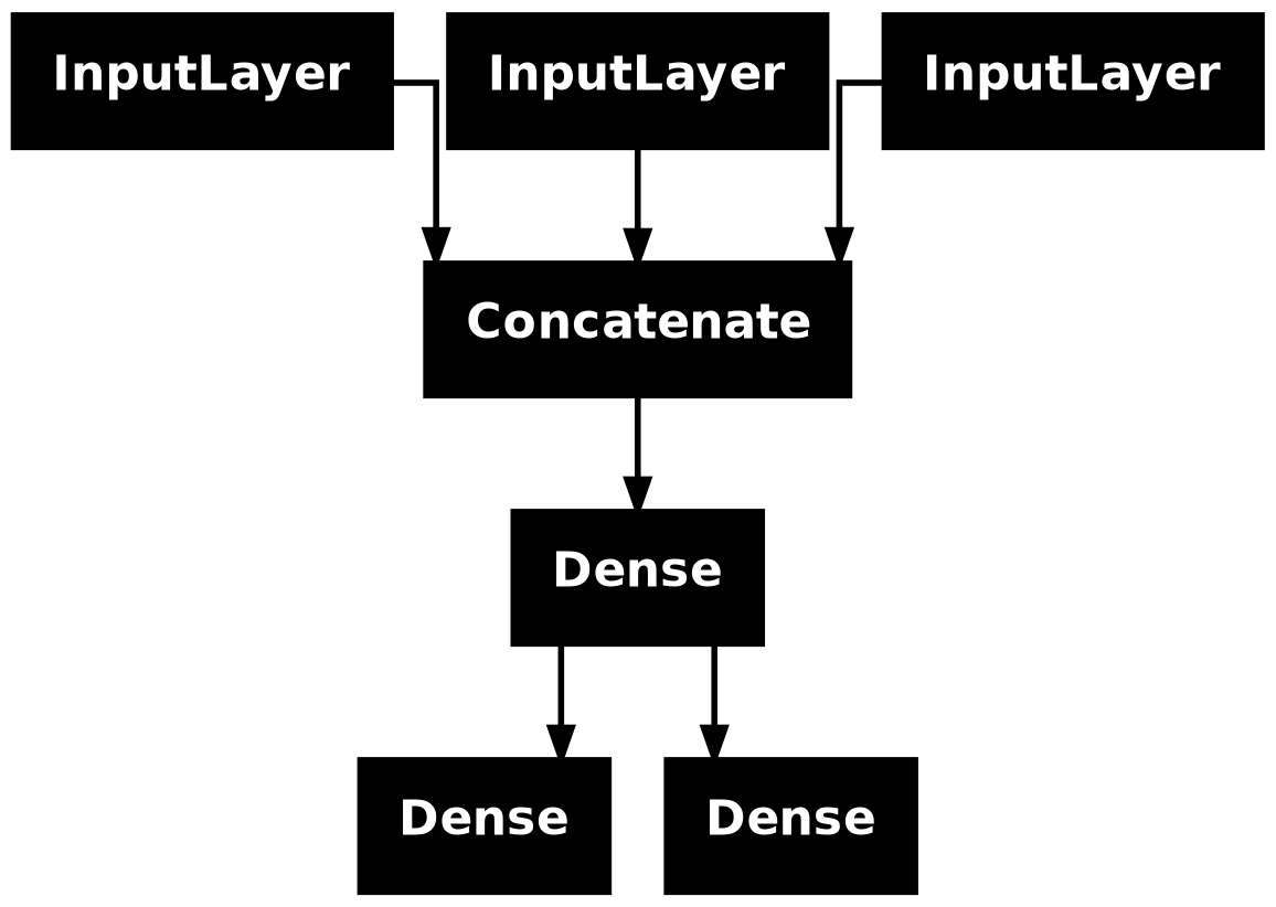
plot() on our ticket classifier modelWe can add to this plot the input and output shapes of each layer in the model, as well as layer names (rather than just layer types), which can be helpful during debugging (figure 7.3):
plot(model, show_shapes = TRUE, show_layer_names = TRUE)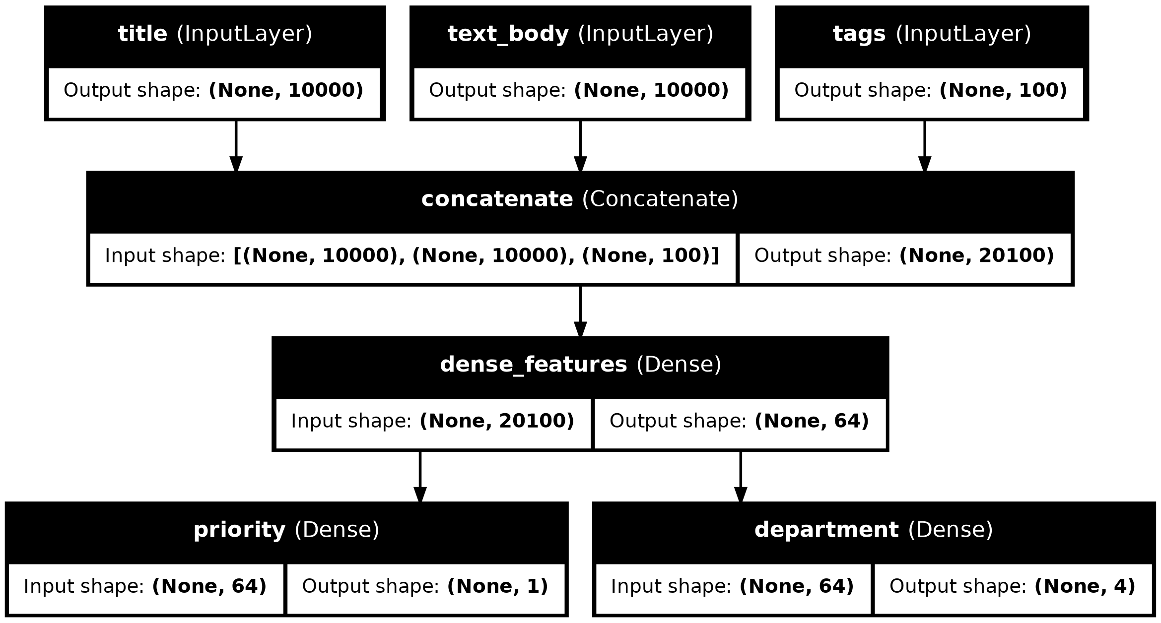
The None in the tensor shapes represents the batch size: this model allows batches of any size. Depending on the context, an unspecified axis size may print as None, NULL, or NA—all three mean the same thing.
Access to layer connectivity also means we can inspect and reuse individual nodes (layer calls) in the graph. The model property model$layers provides the list of layers that make up the model, and for each layer, we can query layer$input and layer$output.
model$layers |> str()List of 7
$ :<InputLayer name=title, built=True>
$ :<InputLayer name=text_body, built=True>
$ :<InputLayer name=tags, built=True>
$ :<Concatenate name=concatenate, built=True>
$ :<Dense name=dense_features, built=True>
[list output truncated]model$layers[[4]]$input |> str()List of 3
$ :<KerasTensor shape=(None, 10000), dtype=float32, sparse=False, ragged=False, name=title>
$ :<KerasTensor shape=(None, 10000), dtype=float32, sparse=False, ragged=False, name=text_body>
$ :<KerasTensor shape=(None, 100), dtype=float32, sparse=False, ragged=False, name=tags>model$layers[[4]]$output |> str()<KerasTensor shape=(None, 20100), dtype=float32, sparse=False, ragged=False, name=keras_tensor_14>This enables us to do feature extraction: creating models that reuse intermediate features from another model.
Let’s say we want to add another output to the model we previously defined: we also want to predict how long a given problem ticket will take to resolve—a kind of difficulty rating. We can do this via a classification layer over three categories: “quick,” “medium,” and “difficult.” We don’t need to re-create and retrain a model from scratch! We can just start from the intermediate features of our previous model, because we have access to them.
1features <- model$layers[[5]]$output
difficulty <- features |>
  layer_dense(3, activation = "softmax", name = "difficulty")

new_model <- keras_model(
  inputs = list(title, text_body, tags),
  outputs = list(priority, department, difficulty)
)layers[[5]] is our intermediate Dense layer
Let’s plot our new model:
plot(new_model, show_shapes = TRUE, show_layer_names = TRUE)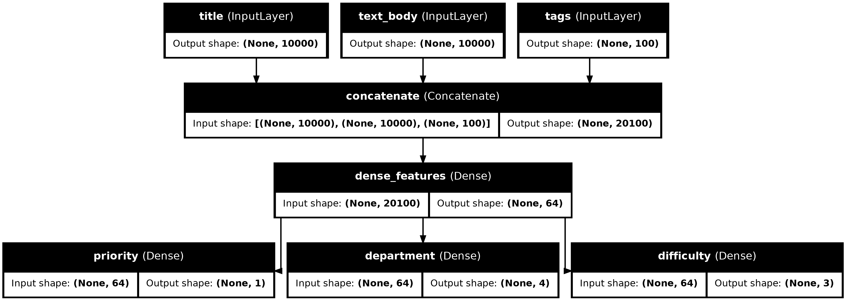
Model classThe last model-building pattern you should know about is the most advanced one: Model subclassing. You learned in chapter 3 how to subclass the Layer class to create custom layers. Subclassing Model is pretty similar:
initialize method, define the layers the model will use.call method, define the forward pass of the model, reusing the layers previously created.Let’s take a look at a simple example: we will reimplement the customer support ticket management model using a Model subclass.
CustomerTicketModel <- new_model_class(
  classname = "CustomerTicketModel",

  initialize = function(num_departments) {
1    super$initialize()
2    self$concat_layer <- layer_concatenate()
    self$mixing_layer <- layer_dense(, 64, activation = "relu")
    self$priority_scorer <- layer_dense(, 1, activation = "sigmoid")
    self$department_classifier <- layer_dense(, num_departments,
                                              activation = "softmax")
  },

3  call = function(inputs) {
    .[title = title, text_body = text_body, tags = tags] <- inputs

    features <- list(title, text_body, tags) |>
      self$concat_layer() |>
      self$mixing_layer()
    priority <- features |> self$priority_scorer()
    department <- features |> self$department_classifier()
    list(priority, department)
  }
)super constructor!
Once we’ve defined the model, we can instantiate it. Note that it will only create its weights the first time we call it on some data—much like Layer subclasses:
model <- CustomerTicketModel(num_departments = 4)
.[priority, department] <- model(list(
  title = title_data,
  text_body = text_body_data,
  tags = tags_data
))
So far, everything looks very similar to Layer subclassing, a workflow you’ve already encountered in chapter 3. What, then, is the difference between a Layer subclass and a Model subclass? It’s simple: a layer is a building block we use to create models, and a model is the top-level object that we will actually train, export for inference, etc. In short, a Model has fit(), evaluate(), and predict() methods. Layers don’t. Other than that, the two classes are virtually identical (another difference is that we can save a model to a file on disk—which we will cover in a few sections).
We can compile and train a Model subclass just like a Sequential or Functional model:
model |> compile(
  optimizer = "adam",
1  loss = c("mean_squared_error", "sparse_categorical_crossentropy"),
  metrics = c("mean_absolute_error", "accuracy")
)
model |> fit(
2  x = list(title = title_data,
           text_body = text_body_data,
           tags = tags_data),
  y = list(priority_data, department_data),
  epochs = 1
)
model |> evaluate(
  x = list(title = title_data,
           text_body = text_body_data,
           tags = tags_data),
  y = list(priority_data, department_data)
)
.[priority_preds, department_preds] <- model |> predict(
  list(title = title_data,
       text_body = text_body_data,
       tags = tags_data)
)The Model subclassing workflow is the most flexible way to build a model: it enables us to build models that cannot be expressed as directed acyclic graphs of layers: imagine, for instance, a model where the call() method uses layers inside a for loop, or even calls them recursively. Anything is possible—you’re in charge.
This freedom comes at a cost: with subclassed models, we are responsible for more of the model logic, which means the potential error surface is much larger. As a result, we will have more debugging work to do. We are developing a new stateful object, not just snapping together LEGO bricks.
Functional and subclassed models are also substantially different in nature: a Functional model is an explicit data structure—a graph of layers, which we can view, inspect, and modify. Meanwhile, a subclassed model is a piece of bytecode: a class with a call() method that contains raw code. This is the source of the subclassing workflow’s flexibility—we can just code up whatever functionality we’d like—but it introduces new limitations.
For instance, because the way layers are connected to each other is hidden inside the body of the call() method, we cannot access that information. Calling print() will not display layer connectivity, and we cannot plot the model topology via plot(model). Likewise, if we have a subclassed model, we cannot access the nodes of the graph of layers to do feature extraction—because there is no graph. Once the model is instantiated, its forward pass becomes a complete black box.
Crucially, choosing one of these patterns—the Sequential model, the Functional API, or Model subclassing—does not lock us out of the others. All models in the Keras API can smoothly interoperate with each other, whether they’re Sequential models, Functional models, or subclassed models written from scratch. They’re all part of the same spectrum of workflows. For instance, we can use a subclassed layer or model in a Functional model.
Classifier <- new_model_class(
  classname = "Classifier",

  initialize = function(num_classes = 2) {
    super$initialize()
    if (num_classes == 2) {
      num_units <- 1
      activation <- "sigmoid"
    } else {
      num_units <- num_classes
      activation <- "softmax"
    }
    self$dense <- layer_dense(, num_units, activation = activation)
  },

  call = function(inputs) {
    self$dense(inputs)
  }
)

classifier <- Classifier(num_classes = 10)

inputs <- keras_input(shape = c(3))
outputs <- inputs |>
  layer_dense(64, activation = "relu") |>
  classifier()
model <- keras_model(inputs = inputs, outputs = outputs)
Conversely, we can use a Functional model as part of a subclassed layer or model.
inputs <- keras_input(shape = c(64))
outputs <- inputs |> layer_dense(1, activation = "sigmoid")
binary_classifier <- keras_model(inputs = inputs, outputs = outputs)

MyModel <- new_model_class(
  classname = "MyModel",

  initialize = function(num_classes = 2) {
    super$initialize()
    self$dense <- layer_dense(units = 64, activation = "relu")
    self$classifier <- binary_classifier
  },

  call = function(inputs) {
    inputs |>
      self$dense() |>
      self$classifier()
  }
)

model <- MyModel()You’ve learned about the spectrum of workflows for building Keras models, from the simplest workflow (the Sequential model) to the most advanced one (model subclassing). When should you use one over the other? Each one has its pros and cons—pick the one most suitable for the job at hand.
In general, the Functional API provides a pretty good tradeoff between ease of use and flexibility. It also gives you direct access to layer connectivity, which is very powerful for use cases such as model plotting or feature extraction. If you can use the Functional API—that is, if your model can be expressed as a directed acyclic graph of layers—we recommend using it over model subclassing.
Going forward, all examples in this book will use the Functional API, simply because all the models we will work with are expressible as graphs of layers. We will, however, make frequent use of subclassed layers. In general, using Functional models that include subclassed layers provides the best of both worlds: high development flexibility while retaining the advantages of the Functional API.
The principle of progressive disclosure of complexity—access to a spectrum of workflows that go from dead easy to arbitrarily flexible, one step at a time—also applies to model training. Keras provides different workflows for training model: it can be as simple as calling fit() on our data or as advanced as writing a new training algorithm from scratch.
You are already familiar with the compile(), fit(), evaluate(), predict() workflow. As a reminder, it looks like the following listing.
compile() / fit() / evaluate() / predict()
1get_mnist_model <- function() {
  inputs <- keras_input(shape = c(28 * 28))
  outputs <- inputs |>
    layer_dense(512, activation = "relu") |>
    layer_dropout(0.5) |>
    layer_dense(10, activation = "softmax")
  keras_model(inputs, outputs)
}

2.[.[images, labels], .[test_images, test_labels]] <- dataset_mnist()
images <- array_reshape(images, c(60000, 28 * 28)) / 255
test_images <- array_reshape(test_images, c(10000, 28 * 28)) / 255
train_images <- images[10001:60000, ]
val_images <- images[1:10000, ]
train_labels <- labels[10001:60000]
val_labels <- labels[1:10000]

3model <- get_mnist_model()
model |> compile(
  optimizer = "adam",
  loss = "sparse_categorical_crossentropy",
  metrics = "accuracy"
)
4model |> fit(
  train_images, train_labels,
  epochs = 3,
  validation_data = list(val_images, val_labels)
)
5test_metrics <- model |> evaluate(test_images, test_labels)
6predictions <- model |> predict(test_images)fit() to train the model, optionally providing validation data to monitor performance on unseen data
evaluate() to compute the loss and metrics on new data
predict() to compute classification probabilities on new data
There are a couple of ways to customize this simple workflow:
fit() method to schedule actions to be taken at specific points during trainingLet’s take a look at these.
Metrics are key to measuring the performance of a model—in particular, to measure the difference between its performance on the training data and its performance on the test data. Commonly used metrics for classification and regression are already part of the built-in metrics family of function; most of the time, those are what you will use. But if you’re doing anything out of the ordinary, you will need to be able to write your own metrics. It’s simple!
A Keras metric is a subclass of the Keras Metric class. Similarly to layers, a metric has an internal state stored in Keras variables. Unlike layers, these variables aren’t updated via backpropagation, so we have to write the state update logic—which happens in the update_state() method. For example, here’s a simple custom metric that measures the root mean squared error (RMSE) with sparse (integer) labels.
Metric class
1metric_sparse_root_mean_squared_error <- new_metric_class(
  classname = "SparseRootMeanSquaredError",

2  initialize = function(name = "rmse", ...) {
    super$initialize(name = name, ...)
    self$sum_sq_error <- self$add_weight(
      name = "sum_sq_error", initializer = "zeros"
    )
    self$total_samples <- self$add_weight(
      name = "total_samples", initializer = "zeros"
    )
  },

3  update_state = function(y_true, y_pred, sample_weight = NULL) {
    .[num_samples, num_classes] <- op_shape(y_pred)
    y_true <- op_one_hot(
      y_true,
      zero_indexed = TRUE,
      num_classes = num_classes
    )
    sse <- op_sum(op_square(y_true - y_pred))
    self$sum_sq_error$assign_add(sse)
    self$total_samples$assign_add(num_samples)
},Metric class
update_state() for integer labels with categorical predictions. The y_true argument is the targets (or labels) for one batch, and y_pred represents the corresponding predictions from the model. To match our MNIST model, we expect categorical predictions and integer labels. Ignore the sample_weight argument; we won’t use it here.
We use the result() method to return the current value of the metric:
  result = function() {
    op_sqrt(op_divide_no_nan(
      self$sum_sq_error,
      self$total_samples
    ))
  },
Meanwhile, we also need to expose a way to reset the metric state without having to re-instantiate it: this enables the same metric objects to be used across different epochs of training or across both training and evaluation. We do this in the reset_state() method:
  reset_state = function() {
    self$sum_sq_error$assign(0)
    self$total_samples$assign(0)
  }
)
Custom metrics can be used just like built-in ones. Let’s test-drive our metric:
model <- get_mnist_model()
model |> compile(
  optimizer = "adam",
  loss = "sparse_categorical_crossentropy",
  metrics = list("accuracy", metric_sparse_root_mean_squared_error())
)
model |> fit(
  train_images, train_labels,
  epochs = 3,
  validation_data = list(val_images, val_labels)
)
test_metrics <- model |> evaluate(test_images, test_labels)
We can now see the fit() progress bar display the RMSE of our model.
Launching a training run on a large dataset for tens of epochs using fit() can be a bit like launching a paper airplane: past the initial impulse, we don’t have any control over its trajectory or its landing spot. If we want to avoid bad outcomes (and thus wasted paper airplanes), it’s smarter to use not a paper plane but a drone that can sense its environment, send data back to its operator, and automatically make steering decisions based on its current state. The Keras callbacks API will help you transform your call to fit() from a paper airplane into a smart, autonomous drone that can self-introspect and dynamically take action.
A callback is an object (a class instance implementing specific methods) that is passed to the model in the call to fit() and that is called by the model at various points during training. It has access to all the available data about the state of the model and its performance, and it can take action: interrupt training, save a model, load a different weight set, or otherwise alter the state of the model.
Here are some examples of ways we can use callbacks:
fit() progress bar you’re familiar with is in fact a callback!The callbacks function family includes a number of built-in callbacks (this is not an exhaustive list):
callback_model_checkpoint()
callback_early_stopping()
callback_learning_rate_scheduler()
callback_reduce_lr_on_plateau()
callback_csv_logger()
Let’s review two of them to give you an idea of how to use them: callback_early_stopping and callback_model_checkpoint.
When we’re training a model, there are many things we can’t predict from the start. In particular, we can’t tell how many epochs will be needed to get to an optimal validation loss. Our examples so far have adopted the strategy of training for enough epochs that we begin overfitting, using the first run to figure out the optimal number of epochs, and then finally launching a new training run from scratch using this optimal number. Of course, this approach is wasteful. A much better way to handle this is to stop training when we measure that the validation loss is no longer improving. This can be achieved using the EarlyStopping callback.
The EarlyStopping callback interrupts training once a target metric being monitored has stopped improving for a fixed number of epochs. For instance, this callback allows us to interrupt training as soon as we start overfitting, thus avoiding having to retrain our model for a smaller number of epochs. This callback is typically used in combination with ModelCheckpoint, which lets us continually save the model during training (and, optionally, save only the current best model so far: the version of the model that achieved the best performance at the end of an epoch).
callbacks argument in the fit() method
1callbacks_list <- list(
2  callback_early_stopping(
3    monitor = "val_accuracy",
4    patience = 1
  ),
5  callback_model_checkpoint(
6    filepath = "checkpoint_path.keras",
7    monitor = "val_loss",
    save_best_only = TRUE
  )
)

model <- get_mnist_model()
model |> compile(
  optimizer = "adam",
  loss = "sparse_categorical_crossentropy",
8  metrics = "accuracy"
)
9model |> fit(
  train_images, train_labels,
  epochs = 10,
  callbacks = callbacks_list,
  validation_data = list(val_images, val_labels)
)callbacks argument in fit(), which takes a list of callbacks. We can pass any number of callbacks.
val_loss has improved, which allows us to keep the best model seen during training.
validation_data to the call to fit().
Note that we can always save models manually after training as well—just call save_model(model, "checkpoint_path.keras"). To reload the model we’ve saved, we use
model <- load_model("checkpoint_path.keras")If we need to take a specific action during training that isn’t covered by one of the built-in callbacks, we can write our own callback. Callbacks are implemented by subclassing the class Callback. We can then implement any number of the following transparently named methods, which are called at various points during training:
These methods are all called with a logs argument, which is a named list containing information about the previous batch, epoch, or training run: training and validation metrics, and so on. The on_epoch_* and on_batch_* methods also take the epoch or batch index as the first argument (an integer).
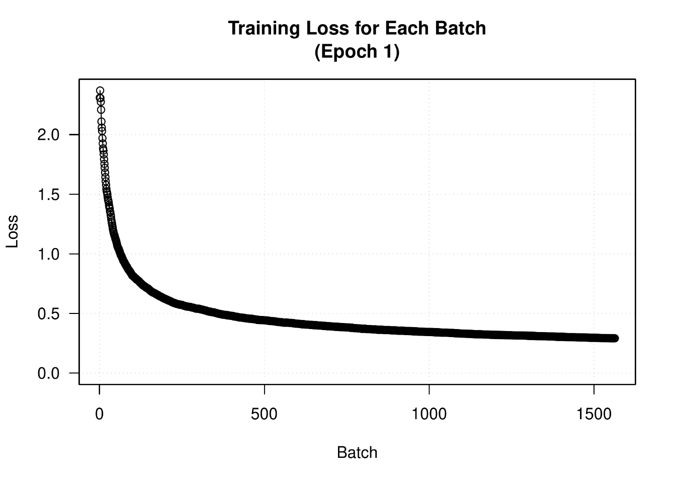
Here’s a simple example callback that saves a list of per-batch loss values during training and plots these values at the end of each epoch.
Callback class
callback_plot_per_batch_loss_history <- new_callback_class(
  classname = "PlotPerBatchLossHistory",

  initialize = function(file = "training_loss.pdf") {
    private$outfile <- file
  },

  on_train_begin = function(logs = NULL) {
    private$plots_dir <- tempfile()
    dir.create(private$plots_dir)
    private$per_batch_losses <-
1      reticulate::py_eval("[]", convert = FALSE)
  },

  on_epoch_begin = function(epoch, logs = NULL) {
    private$per_batch_losses$clear()
  },

  on_batch_end = function(batch, logs = NULL) {
    private$per_batch_losses$append(logs$loss)
  },

  on_epoch_end = function(epoch, logs = NULL) {
    losses <- as.numeric(reticulate::py_to_r(private$per_batch_losses))

    filename <- sprintf("epoch_%04i.pdf", epoch)
    filepath <- file.path(private$plots_dir, filename)

    pdf(filepath, width = 7, height = 5)
    on.exit(dev.off())

    plot(losses, type = "o",
         ylim = c(0, max(losses)),
         panel.first = grid(),
         main = sprintf("Training Loss for Each Batch\n(Epoch %i)", epoch),
         xlab = "Batch", ylab = "Loss")
  },

  on_train_end = function(logs) {
    private$per_batch_losses <- NULL
    plots <- sort(list.files(private$plots_dir, full.names = TRUE))
    qpdf::pdf_combine(plots, private$outfile)
    unlink(private$plots_dir, recursive = TRUE)
  }
)Let’s test-drive it:
model <- get_mnist_model()
model |> compile(
  optimizer = "adam",
  loss = "sparse_categorical_crossentropy",
  metrics = "accuracy"
)
model |> fit(
  train_images, train_labels,
  epochs = 10,
  callbacks = list(callback_plot_per_batch_loss_history()),
  validation_data = list(val_images, val_labels)
)
We get plots that look like figure 7.5.
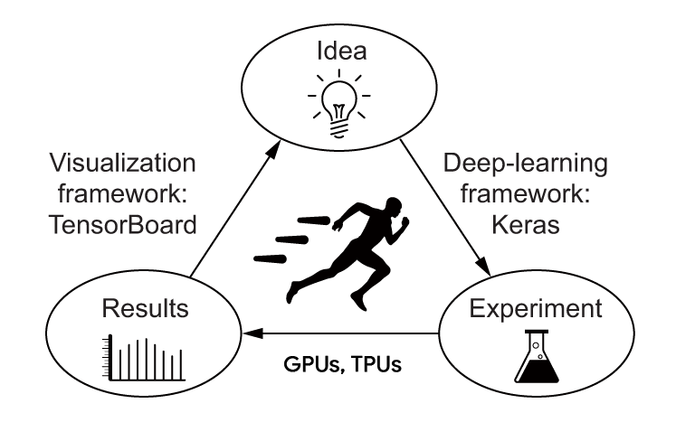
To do good research and develop good models, we need rich, frequent feedback about what’s going on inside our models during our experiments. That’s the point of running experiments: to get information about how well a model performs—as much information as possible. Making progress is an iterative process: we start with an idea and express it as an experiment, attempting to validate or invalidate it. We run this experiment and process the information it generates, as shown in figure 7.6. This inspires our next idea. The more iterations of this loop we can run, the more refined and powerful our ideas become. Keras helps us go from idea to experiment in the least possible time, and fast GPUs can help us get from experiment to result as quickly as possible. But what about processing the experiment results? That’s where TensorBoard comes in.
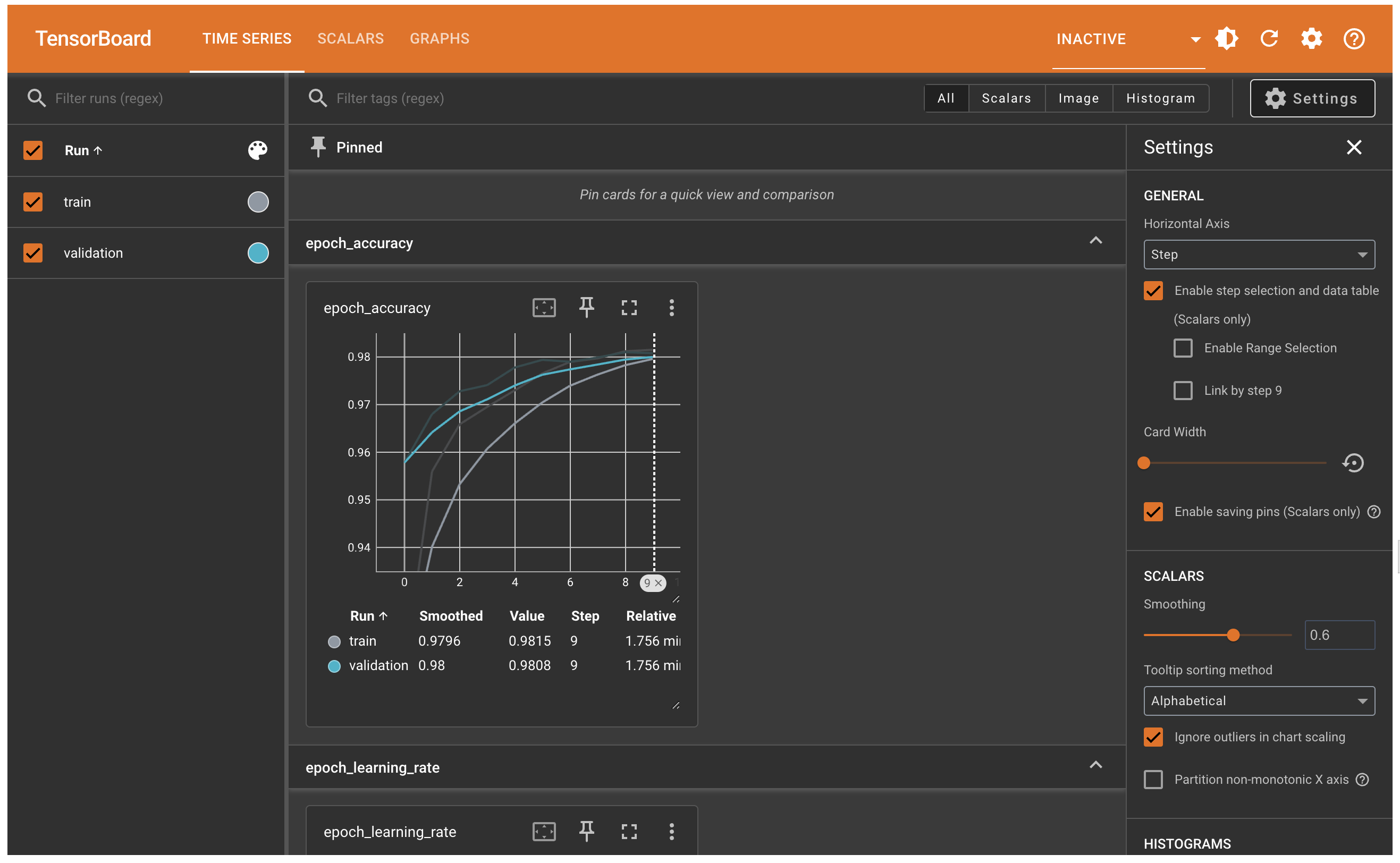
TensorBoard is a browser-based application that we can run locally. It’s the best way to monitor everything that goes on inside our model during training. With TensorBoard, we can
If we’re monitoring more information than just the model’s final loss, we can develop a clearer vision of what the model does and doesn’t do, and we can make progress more quickly.
The easiest way to use TensorBoard with a Keras model and the fit() method is with callback_tensorboard(). In the simplest case, we just specify where we want the callback to write logs, and we’re good to go:
model <- get_mnist_model()
model |> compile(
  optimizer = "adam",
  loss = "sparse_categorical_crossentropy",
  metrics = "accuracy"
)

model |> fit(
  train_images, train_labels,
  epochs = 10,
  validation_data = list(val_images, val_labels),
  callbacks = c(
    callback_tensorboard(
      log_dir = "./full_path_to_your_log_dir"
    )
  )
)
Once the model starts running, it will write logs at the target location. If you are running your R script on a local machine, you can launch the local TensorBoard server using the following function:
# Load TensorBoard in R
tensorboard(log_dir = "./full_path_to_your_log_dir")
In the TensorBoard interface, you can monitor live graphs of your training and evaluation metrics, as shown in figure 7.7.
The fit() workflow strikes a nice balance between ease of use and flexibility. It’s what you will use most of the time. However, it isn’t meant to support everything a deep learning researcher may want to do—even with custom metrics, custom losses, and custom callbacks.
After all, the built-in fit() workflow is solely focused on supervised learning: a setup where there are known targets (also called labels or annotations) associated with input data and where we compute our loss as a function of these targets and the model’s predictions. However, not every form of machine learning falls into this category. There are other setups where no explicit targets are present, such as generative learning (which we will introduce in chapter 16), self-supervised learning (where targets are obtained from the inputs), and reinforcement learning (where learning is driven by occasional “rewards”—much like training a dog). And even if you’re doing regular supervised learning, as a researcher, you may want to add some novel bells and whistles that require low-level flexibility.
Whenever you find yourself in a situation where the built-in fit() is not enough, you will need to write your own custom training logic. You’ve already seen simple examples of low-level training loops in chapters 2 and 3. As a reminder, the contents of a typical training loop look like this:
forward pass” (compute the model’s output) to obtain a loss value for the current batch of data.These steps are repeated for as many batches as necessary. This is essentially what fit() does under the hood. In this section, you will learn to reimplement fit() from scratch, which will give you all the knowledge you need to write any training algorithm you may come up with.
Let’s go over the details. Throughout the next few sections, you’ll work your way up to writing a fully featured custom training loop in TensorFlow, PyTorch, and JAX.
In the low-level training loop examples you’ve seen so far, step 1 (the forward pass) was done via predictions = model(inputs), and step 2 (retrieving the gradients computed by the gradient tape) was done via a backend-specific API, such as
gradients <- tape$gradient(loss, model$weights) in TensorFlowloss$backward() in PyTorchjax$value_and_grad() in JAXIn the general case, we need to take two subtleties into account. Some Keras layers, such as the Dropout layer, have different behaviors during training and during inference (when we use them to generate predictions). Such layers expose a training boolean argument in their call() method. Calling dropout(inputs, training=TRUE) will drop some activation entries, and calling dropout(inputs, training=FALSE) does nothing. By extension, Functional models and Sequential models also expose this training argument in their call() methods. Remember to pass training=TRUE when you call a Keras model during the forward pass! Our forward pass thus becomes predictions = model(inputs, training=TRUE).
In addition, note that when we retrieve the gradients of the weights of our model, we should not use model$weights, but rather model$trainable_weights. Indeed, layers and models own two kinds of weights:
Dense layerAmong Keras built-in layers, the only layer that features nontrainable weights is the BatchNormalization layer, which we will introduce in chapter 9. The BatchNormalization layer needs nontrainable weights to track information about the mean and standard deviation of the data that passes through it, to perform an online approximation of feature normalization (a concept you learned about in chapters 4 and 6).
Taking into account these two details, a supervised learning training step ends up looking like this, in pseudo-code:
This snippet is pseudo-code rather than real code because it includes an imaginary function, get_gradients_of(). In reality, retrieving gradients is done in a way that is specific to our current backend: JAX, TensorFlow, or PyTorch.
Let’s use what you learned about each framework in chapter 3 to implement a real version of this train_step() function. We’ll start with TensorFlow and PyTorch because these two make the job relatively easy. We’ll end with JAX, which is quite a bit more complex.
TensorFlow lets us write code that looks pretty much like our pseudo-code snippet. The only difference is that the forward pass should take place inside a GradientTape scope. We can then use the tape object to retrieve the gradients:
library(tensorflow, exclude = c("set_random_seed", "shape"))
library(keras3)

use_backend("tensorflow")
get_mnist_model <- function() {
inputs <- keras_input(shape = c(28 * 28))
outputs <- inputs |>
layer_dense(512, activation = "relu") |>
layer_dropout(0.5) |>
layer_dense(10, activation = "softmax")
keras_model(inputs, outputs)
}model <- get_mnist_model()
loss_fn <- loss_sparse_categorical_crossentropy()
optimizer <- optimizer_adam()
train_step <- function(inputs, targets) {
1 with(tf$GradientTape() %as% tape, {
2 predictions <- model(inputs, training = TRUE)
loss <- loss_fn(targets, predictions)
})
3 gradients <- tape$gradient(loss, model$trainable_weights)
4 optimizer$apply(gradients, model$trainable_weights)
loss
}GradientTape
Let’s run it for a single step:
batch_size <- 32
inputs <- train_images[1:batch_size, ]
targets <- train_labels[1:batch_size]
loss <- train_step(inputs, targets)
loss
tf.Tensor(2.5361915, shape=(), dtype=float32)Easy enough! Let’s do PyTorch next.
When we use the PyTorch backend, all of our Keras layers and models inherit from the PyTorch torch$nn$Module class and expose the native Module API. As a result, our model, its trainable weights, and our loss tensor are all aware of each other and interact via three methods: loss$backward(), weight$value$grad, and model$zero_grad().
As a reminder from chapter 3, the mental model to keep in mind is as follows:
$backward() on any given scalar node of this graph (like our loss) will run the graph backward starting from that node, automatically populating a tensor$grad attribute on all tensors involved (if they satisfy requires_grad=TRUE) containing the gradient of the output node with respect to that tensor. In particular, it will populate the grad attribute of our trainable parameters.tensor$grad attribute, we should call tensor$grad <- NULL on all our tensors. Because it would be a bit cumbersome to do this on all model variables individually, we can just do it at the model level via model$zero_grad()—the zero_grad() call will propagate to all variables tracked by the model. Clearing gradients is critical because calls to backward() are additive: if we don’t clear the gradients at each step, the gradient values would accumulate, and training would not proceed.Let’s chain these steps:
library(reticulate)
library(keras3)

use_backend("torch")
torch <- import("torch")
loss_fn <- loss_sparse_categorical_crossentropy()
optimizer <- optimizer_adam()
model <- get_mnist_model()
train_step <- function(inputs, targets) {
1 predictions <- model(inputs, training = TRUE)
loss <- loss_fn(targets, predictions)
2 loss$backward()
gradients <- model$trainable_weights |>
3 lapply(\(weight) weight$value$grad)
with(torch$no_grad(), {
optimizer$apply(gradients, model$trainable_weights)
4 })
5 model$zero_grad()
loss
}weight$value is the PyTorch tensor that contains the variable’s value.
no_grad() scope.
Let’s run it for a single step:
batch_size <- 32
inputs <- train_images[1:batch_size, ]
targets <- train_labels[1:batch_size]
loss <- train_step(inputs, targets)
loss
tensor(2.3919, device='cuda:0', grad_fn=<WhereBackward0>)That wasn’t too difficult! Now, let’s move on to JAX.
When it comes to low-level training code, JAX tends to be the most complex of the three backends, because of its fully stateless nature. Statelessness makes JAX highly performant and scalable by enabling compilation and automatic performance optimizations. However, writing stateless code requires us to jump through some hoops.
Because the gradient function is obtained via metaprogramming, we first need to define the function that returns our loss. Further, this function needs to be stateless, so it needs to take as arguments all the variables it’s going to be using, and it needs to return the value of any variable it has updated. Remember those nontrainable weights that can get modified during the forward pass? Those are the variables we need to return.
To make it easier to work with the stateless programming paradigm of JAX, Keras models have a stateless forward-pass method: the stateless_call() method. It behaves just like call(), except that
inputs and training arguments.It works like this:
.[outputs, non_trainable_weights] <- model$stateless_call(
    inputs, trainable_weights, non_trainable_weights
)
We can use stateless_call() to implement our JAX loss function. Because the loss function also computes updates for all nontrainable variables, we name it compute_loss_and_updates():
library(reticulate)
library(keras3)

use_backend("jax")
jax <- import("jax")
model <- get_mnist_model()
model$build(shape(28 * 28))
loss_fn <- loss_sparse_categorical_crossentropy()
compute_loss_and_updates <- function(
1 trainable_variables,
non_trainable_variables,
inputs,
targets
) {
.[outputs, non_trainable_variables] <-
2 model$stateless_call(
trainable_variables,
non_trainable_variables,
inputs,
training = TRUE
)
loss <- loss_fn(targets, outputs)
3 list(loss, non_trainable_variables)
}stateless_call()
Once we have this compute_loss_and_updates() function, we can pass it to jax$value_and_grad() to obtain the gradient-computation:
grad_fn <- jax$value_and_grad(fn)
.[loss, gradients] <- grad_fn(...)
Now, there’s just a small problem. Both jax$grad() and jax$value_and_grad() require fn to return a scalar value only. Our compute_loss_and_updates() function returns a scalar value as its first output, but it also returns the new value for the nontrainable weights. Remember what you learned in chapter 3? The solution is to pass a has_aux argument to grad() or value_and_grad(), like this:
grad_fn <- jax$value_and_grad(compute_loss_and_updates, has_aux = TRUE)We use it like this:
.[.[loss, non_trainable_weights], gradients] <- grad_fn(
    trainable_variables, non_trainable_variables, inputs, targets
)
Ok, that was a lot of JAXiness. But now we’ve got almost everything to assemble our JAX training step. We just need the last piece of the puzzle: optimizer$apply().
When we wrote our first basic training step in TensorFlow at the beginning of chapter 2, we wrote an update step function that looked like this:
learning_rate <- 1e-3

update_weights <- function(gradients, weights) {
  Map(\(w, g) w$assign(w - g * learning_rate),
      weights, gradients)
}
This corresponds to what Keras’s optimizer_sgd() would do. However, every other optimizer in the Keras API is somewhat more complex than that and keeps track of auxiliary variables that help speed up training—in particular, most optimizers use some form of momentum, which you learned about in chapter 2. These extra variables are updated at each step of training, and in the JAX world, that means we need to get our hands on a stateless function that takes these variables as arguments and returns their new value.
To make this easy, Keras makes available the stateless_apply() method on all optimizers. It works like this:
.[trainable_variables, optimizer_variables] <- optimizer$stateless_apply(
    optimizer_variables, grads, trainable_variables
)
Now we have enough to assemble an end-to-end training step:
optimizer <- optimizer_adam()
optimizer$build(model$trainable_variables)

1train_step <- function(state, inputs, targets) {
  .[trainable_variables, non_trainable_variables, optimizer_variables] <-
2    state

3  .[.[loss, non_trainable_variables], grads] <- grad_fn(
    trainable_variables, non_trainable_variables,
    inputs, targets
  )
4  .[trainable_variables, optimizer_variables] <- optimizer$stateless_apply(
    optimizer_variables, grads, trainable_variables
  )
5  new_state <- list(
    trainable_variables,
    non_trainable_variables,
    optimizer_variables
  )
  list(loss, new_state)
}Let’s run it for a single step:
batch_size <- 32
inputs <- train_images[1:batch_size, ]
targets <- train_labels[1:batch_size]

trainable_variables <- model$trainable_variables |> lapply(\(w) w$value)
non_trainable_variables <-
  model$non_trainable_variables |> lapply(\(w) w$value)
optimizer_variables <- optimizer$variables |> lapply(\(w) w$value)

state <- list(trainable_variables, non_trainable_variables, optimizer_variables)
.[loss, state] <- train_step(state, inputs, targets)
loss
Array(2.393485, dtype=float32)It’s definitely a bit more work than TensorFlow and PyTorch, but the speed and scalability benefits of JAX more than make up for it. Next, let’s take a look at another important element of a custom training loop: metrics.
In a low-level training loop, you will probably want to use Keras metrics (custom ones or the built-in ones). You’ve already learned about the metrics API: simply call update_state(y_true, y_pred) for each batch of targets and predictions and then use result() to query the current metric value:
metric <- metric_sparse_categorical_accuracy()
targets <- op_array(c(0, 1, 2), dtype = "int32")
predictions <- op_array(rbind(c(1, 0, 0), c(0, 1, 0), c(0, 0, 1)))
metric$update_state(targets, predictions)
current_result <- metric$result()
cat(sprintf("result: %.2f\n", current_result))
result: 1.00You may also need to track the average of a scalar value, such as the model’s loss. You can do this via metric_mean():
mean_tracker <- metric_mean()
for(value in 0:4) {
  value <- op_array(value)
  mean_tracker$update_state(value)
}
cat(sprintf("Mean of values: %.2f\n", mean_tracker$result()))
Mean of values: 2.00Remember to use metric$reset_state() when you want to reset the current results (at the start of a training epoch or at the start of evaluation).
Now, if you’re using JAX, state-modifying methods like update_state() or reset_state() can’t be used inside a stateless function. Instead, you can use the stateless metrics API, which is similar to the model$stateless_call() and optimizer$stateless_apply() methods you’ve already learned about. Here’s how it works:
metric <- metric_sparse_categorical_accuracy()
targets <- op_array(c(0, 1, 2), dtype = "int32")
predictions <-  op_array(rbind(c(1, 0, 0), c(0, 1, 0), c(0, 0, 1)))

1metric_variables <- metric$variables
2metric_variables <- metric$stateless_update_state(
  metric_variables, targets, predictions
)
3current_result <- metric$stateless_result(metric_variables)
cat(sprintf("result: %.2f\n", current_result))

4metric_variables <- metric$stateless_reset_state()result: 1.00fit() with a custom training loopIn the previous sections, we wrote our own training logic entirely from scratch. Doing so provides the most flexibility, but we end up writing a lot of code while simultaneously missing out on many convenient features of fit(), such as callbacks, performance optimizations, and built-in support for distributed training.
What if we need a custom training algorithm, but we still want to use the power of the built-in Keras training loop? There’s actually a middle ground between fit() and a training loop written from scratch: we can provide a custom training step function and let the framework do the rest.
We can do this by overriding the train_step() method of the Model class. This is the function that is called by fit() for every batch of data. We can then call fit() as usual—and it will run our learning algorithm under the hood.
Here’s how it works:
Model.train_step() method. Its contents are nearly identical to what we used in the previous section.Note the following:
Sequential models, Functional API models, or subclassed models.tf_function() or jax$jit() when you override train_step()—the framework does it for you.Let’s start by coding a custom TensorFlow train step:
loss_fn <- loss_sparse_categorical_crossentropy()
1loss_tracker <- metric_mean(name="loss")

CustomModel <- new_model_class(
  "CustomModel",

2  train_step = function(data) {
    .[inputs, targets] <- data
    with(tf$GradientTape() %as% tape, {
3      predictions <- self(inputs, training = TRUE)
      loss <- loss_fn(targets, predictions)
    })
    gradients <- tape$gradient(loss, model$trainable_weights)
    self$optimizer$apply(gradients, model$trainable_weights)

4    loss_tracker$update_state(loss)
5    list("loss" = loss_tracker$result())
  },

  metrics = active_property(\() {
6    list(loss_tracker)
  })
)Metric object to track the average of per-batch losses during training and evaluation
train_step() method
self(inputs, training=TRUE) instead of model(inputs, training=TRUE) because our model is the class itself.
reset_state() on it at the start of each epoch and at the start of a call to evaluate()—so we don’t have to do it by hand. Any metric you want to reset across epochs should be listed here.
We can now instantiate our custom model, compile it (we only pass the optimizer, because the loss is already defined outside of the model), and train it using fit() as usual. Let’s put the model definition in its own reusable function:
get_custom_model <- function() {
  inputs <- keras_input(shape = (28 * 28))
  outputs <- inputs |>
    layer_dense(512, activation = "relu") |>
    layer_dropout(0.5) |>
    layer_dense(10, activation = "softmax")
  model <- CustomModel(inputs, outputs)
  model |> compile(optimizer = optimizer_adam())
  model
}
Let’s give it a whirl:
model <- get_custom_model()
model |> fit(train_images, train_labels, epochs=3)fit() with PyTorchNext, the PyTorch version:
loss_fn <- loss_sparse_categorical_crossentropy()
loss_tracker <- metric_mean(name = "loss")

CustomModel <- new_model_class(
  "CustomModel",

  train_step = function(data) {
    .[inputs, targets] <- data
1    predictions <- self(inputs, training = TRUE)
    loss <- loss_fn(targets, predictions)

2    loss$backward()
    trainable_weights <- self$trainable_weights
    gradients <- trainable_weights |> lapply(\(v) v$value$grad)

    with(torch$no_grad(), {
3      self$optimizer$apply(gradients, trainable_weights)
    })

4    loss_tracker$update_state(loss)
5    list(loss = loss_tracker$result())
  },

  metrics = active_property(\() {
    list(loss_tracker)
  })
)Let’s try it:
model <- get_custom_model()
model |> fit(train_images, train_labels, epochs=3)fit() with JAXFinally, let’s write the JAX version. First we need to define a compute_loss_and_updates() method, similar to the compute_loss_and_updates() function we used in our custom training step example:
loss_fn <- loss_sparse_categorical_crossentropy()

CustomModel <- new_model_class(
  "CustomModel",

  compute_loss_and_updates = function(
    trainable_variables,
    non_trainable_variables,
    inputs,
    targets,
    training = FALSE
  ) {
    .[predictions, non_trainable_variables] <- self$stateless_call(
      trainable_variables,
      non_trainable_variables,
      inputs,
      training = training
    )
    loss <- loss_fn(targets, predictions)
1    list(loss, non_trainable_variables)
},Note that we aren’t computing a moving average of the loss as we did for the other two backends. Instead, we just return the per-batch loss value, which is less useful. We do this to simplify metric state management in the example: the code would get very verbose if we included it (you will learn about metric management in the next section):
1  train_step = function(state, data) {
    .[
      trainable_variables,
      non_trainable_variables,
      optimizer_variables,
      metrics_variables
    ] <- state
    .[inputs, targets] <- data

2    grad_fn <- jax$value_and_grad(
      self$compute_loss_and_updates,
      has_aux = TRUE
    )

3    .[.[loss, non_trainable_variables], grads] <- grad_fn(
      trainable_variables,
      non_trainable_variables,
      inputs,
      targets,
      training = TRUE
    )

4    .[trainable_variables, optimizer_variables] <-
      self$optimizer$stateless_apply(
        optimizer_variables,
        grads,
        trainable_variables
      )

5    logs <- list(loss = loss)
    new_state <- list(
      trainable_variables,
      non_trainable_variables,
      optimizer_variables,
      metrics_variables
    )
6    list(logs, new_state)
  }
)metrics_variables are part of it, although we won’t use them here.
Let’s try it out:
model <- get_custom_model()
model |> fit(train_images, train_labels, epochs=3)Finally, what about the loss and metrics that we can pass to compile()? After we’ve called compile(), we get access to
self$compute_loss()—Combines the loss function we passed to compile() with regularization losses that may be added by certain layers.self$metrics—The list of metrics we passed to compile(). Note that it also includes a metric that tracks the loss.train_step() metrics handling with TensorFlowHere’s what it looks like with TensorFlow:
CustomModel <- new_model_class(
  "CustomModel",
  train_step = function(data) {
    .[inputs, targets] <- data
    with(tf$GradientTape() %as% tape, {
      predictions <- self(inputs, training = TRUE)
1      loss <- self$compute_loss(y=targets, y_pred=predictions)
    })
    gradients <- tape$gradient(loss, self$trainable_weights)
    self$optimizer$apply(gradients, self$trainable_weights)

    logs <- list()
2    for (metric in self$metrics) {
      if (metric$name == "loss")
        metric$update_state(loss)
      else
        metric$update_state(targets, predictions)

      logs[[metric$name]] <- metric$result()
    }

3    logs
  }
)self$compute_loss
Let’s try it:
get_custom_model <- function() {
  inputs <- keras_input(shape = (28 * 28))
  outputs <- inputs |>
    layer_dense(512, activation = "relu") |>
    layer_dropout(0.5) |>
    layer_dense(10, activation = "softmax")

  model <- CustomModel(inputs, outputs)
  model |> compile(
    optimizer = optimizer_adam(),
    loss = loss_sparse_categorical_crossentropy(),
    metrics = c(metric_sparse_categorical_accuracy())
  )
  model
}

model <- get_custom_model()
model |> fit(train_images, train_labels, epochs = 3)train_step() metrics handling with PyTorchAnd here’s what it looks like with PyTorch—it’s exactly the same code change!
CustomModel <- new_model_class(
  "CustomModel",

  train_step = function(data) {
    .[inputs, targets] <- data
    predictions <- self(inputs, training = TRUE)
    loss <- self$compute_loss(y = targets, y_pred = predictions)

    loss$backward()
    trainable_weights <- self$trainable_weights
    gradients <- trainable_weights |> lapply(\(v) v$value$grad)

    with(torch$no_grad(), {
      self$optimizer$apply(gradients, trainable_weights)
    })

    logs <- list()
    for (metric in self$metrics) {
      if (metric$name == "loss")
        metric$update_state(loss)
      else
        metric$update_state(targets, predictions)

      logs[[metric$name]] <- metric$result()
    }

    logs
  }
)
Let’s see how it runs:
model <- get_custom_model()
model |> fit(train_images, train_labels, epochs = 3)train_step() metrics handling with JAXFinally, here’s what it looks like with JAX. To start with, we can use compute_loss() in our compute_loss_and_updates() method to hit the loss passed to compile():
CustomModel <- new_model_class(
  "CustomModel",
  compute_loss_and_updates = function(
    trainable_variables,
    non_trainable_variables,
    inputs,
    targets,
    training = FALSE
  ) {
    .[predictions, non_trainable_variables] <-
      self$stateless_call(
        trainable_variables,
        non_trainable_variables,
        inputs,
        training = training
      )
    loss <- self$compute_loss(y = targets, y_pred = predictions)
    tuple(loss, tuple(predictions, non_trainable_variables))
  },
Next up: metric management. As usual, it’s a tad more complicated due to JAX’s statelessness requirements:
  train_step = function(self, state, data) {
    .[
      trainable_variables,
      non_trainable_variables,
      optimizer_variables,
      metrics_variables
1    ] <- state
    .[inputs, targets] <- data

    grad_fn <-
      jax$value_and_grad(self$compute_loss_and_updates, has_aux = TRUE)

    .[.[loss, .[predictions, non_trainable_variables]], grads] <-
      grad_fn(
        trainable_variables,
        non_trainable_variables,
        inputs,
        targets,
        training = TRUE
      )

    .[trainable_variables, optimizer_variables] <-
      self$optimizer$stateless_apply(
        optimizer_variables,
        grads,
        trainable_variables
      )

    logs <- new_metrics_vars <- list()
2    for (metric in self$metrics) {
3      this_metric_vars <- metrics_variables[seq(
        from = length(new_metrics_vars) + 1,
        along.with = metric$variables
      )]
4      this_metric_vars <- if (metric$name == "loss") {
        metric$stateless_update_state(this_metric_vars, loss)
      } else {
        metric$stateless_update_state(this_metric_vars, targets, predictions)
      }
      logs[[metric$name]] <- metric$stateless_result(this_metric_vars)
5      new_metrics_vars <- c(new_metrics_vars, this_metric_vars)
    }

    new_state <- list(
      trainable_variables,
      non_trainable_variables,
      optimizer_variables,
6      new_metrics_vars
    )
    list(logs, new_state)
  }
)That was a lot of information, but by now you know enough to use Keras to do almost anything!
Sequential class, via the Functional API, or by subclassing the Model class. Most of the time, you’ll be using the Functional API.fit() and evaluate() methods.fit() and automatically take action based on the state of the model.fit() does by overriding the train_step() method, using APIs from your backend of choice—JAX, TensorFlow, or PyTorch.fit(), you can also write your own training loops entirely from scratch, in a backend-native way. This is useful for researchers implementing brand-new training algorithms.