

library(keras3)

.[.[train_images, train_labels], .] <- dataset_mnist()
train_images <- array_reshape(train_images / 255, c(60000, 28 * 28))

runif_array <- \(dim) array(runif(prod(dim)), dim)

noise_channels <- runif_array(dim(train_images))
train_images_with_noise_channels <- cbind(train_images, noise_channels)

zeros_channels <- array(0, dim(train_images))
train_images_with_zeros_channels <- cbind(train_images, zeros_channels)5 Fundamentals of machine learning
This chapter covers
- Understanding the tension between generalization and optimization, the fundamental problem in machine learning
- Evaluation methods for machine learning models
- Best practices to improve model fitting
- Best practices to achieve better generalization
After the three practical examples in chapter 4, you should be starting to feel familiar with how to approach classification and regression problems using neural networks, and you’ve witnessed the central problem of machine learning: overfitting. This chapter will formalize some of your new intuition about machine learning into a solid conceptual framework, highlighting the importance of accurate model evaluation and the balance between training and generalization.
5.1 Generalization: The goal of machine learning
In the three examples presented in chapter 4—predicting movie reviews, topic classification, and house-price regression—we split the data into a training set, a validation set, and a test set. The reason not to evaluate the models on the same data they were trained on quickly became evident: after just a few epochs, performance on never-before-seen data started diverging from performance on the training data, which always improves as training progresses. The models started to overfit. Overfitting happens in every machine learning problem.
The fundamental problem in machine learning is the tension between optimization and generalization. Optimization refers to the process of adjusting a model to get the best performance possible on the training data (the learning in machine learning), whereas generalization refers to how well the trained model performs on data it has never seen before. The goal of the game is to get good generalization, of course, but we don’t control generalization; we can only fit the model to its training data. If we do that too well, overfitting kicks in and generalization suffers.
But what causes overfitting? How can we achieve good generalization?
5.1.1 Underfitting and overfitting
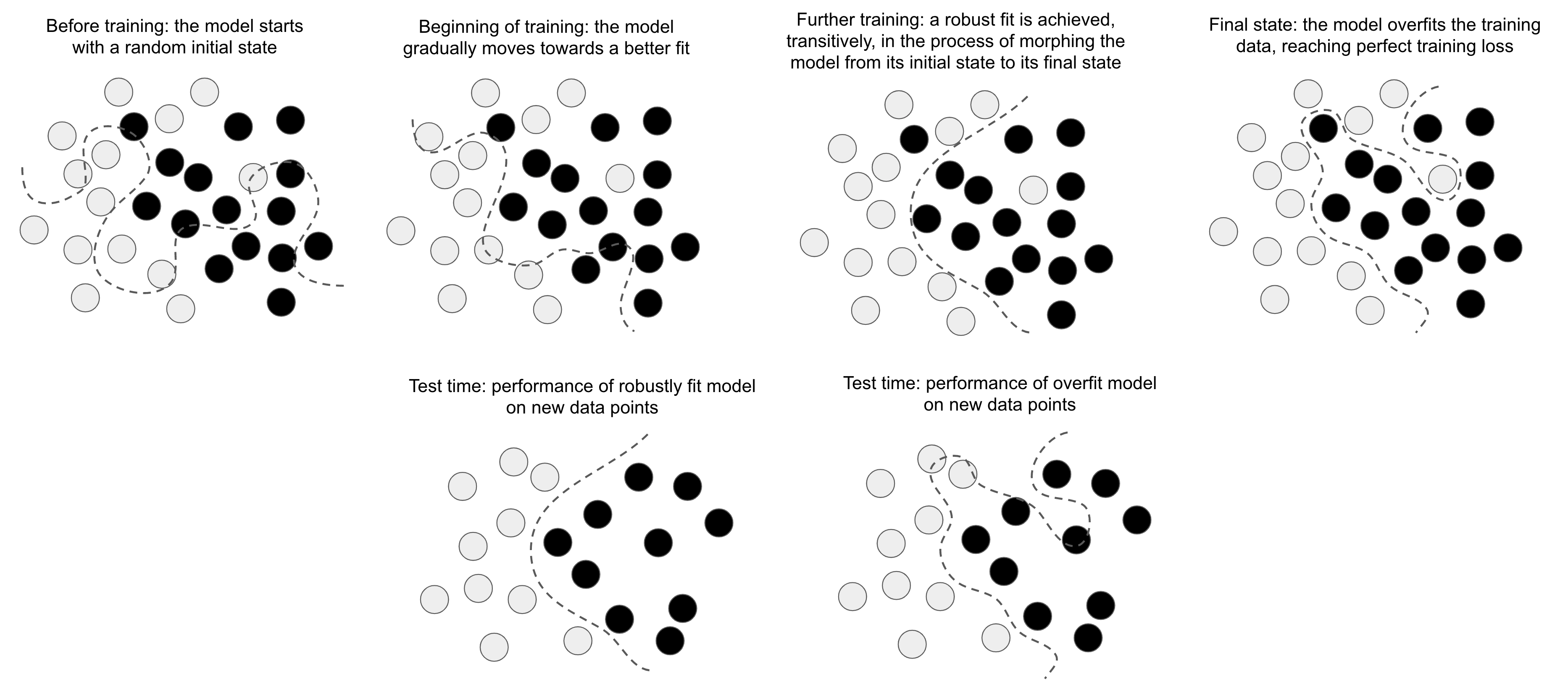
For all the models you saw in the previous chapter, performance on the held-out validation data initially improved as training went on and then inevitably peaked after a while. This pattern (illustrated in figure 5.1) is universal. You’ll see it with any model type and any dataset.
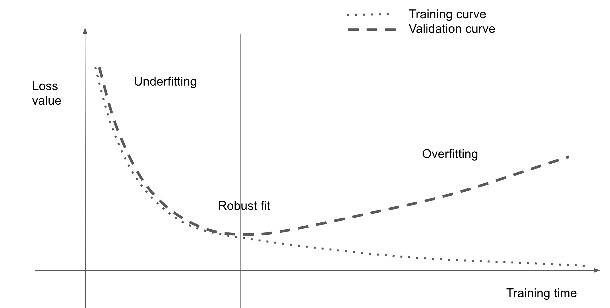
At the beginning of training, optimization and generalization are correlated: the lower the loss on training data, the lower the loss on test data. While this is happening, your model is said to be underfit: there is still progress to be made; the network hasn’t yet modeled all relevant patterns in the training data. But after a certain number of iterations on the training data, generalization stops improving, and validation metrics stall and then begin to degrade: the model is starting to overfit. That is, it’s beginning to learn patterns that are specific to the training data but that are misleading or irrelevant when it comes to new data.
Overfitting is particularly likely to occur when your data is noisy, if it involves uncertainty, or if it includes rare features. Let’s look at concrete examples.
5.1.1.1 Noisy training data
In real-world datasets, it’s fairly common for some inputs to be invalid. Perhaps an MNIST digit is an all-black image, for instance, or something like figure 5.2.
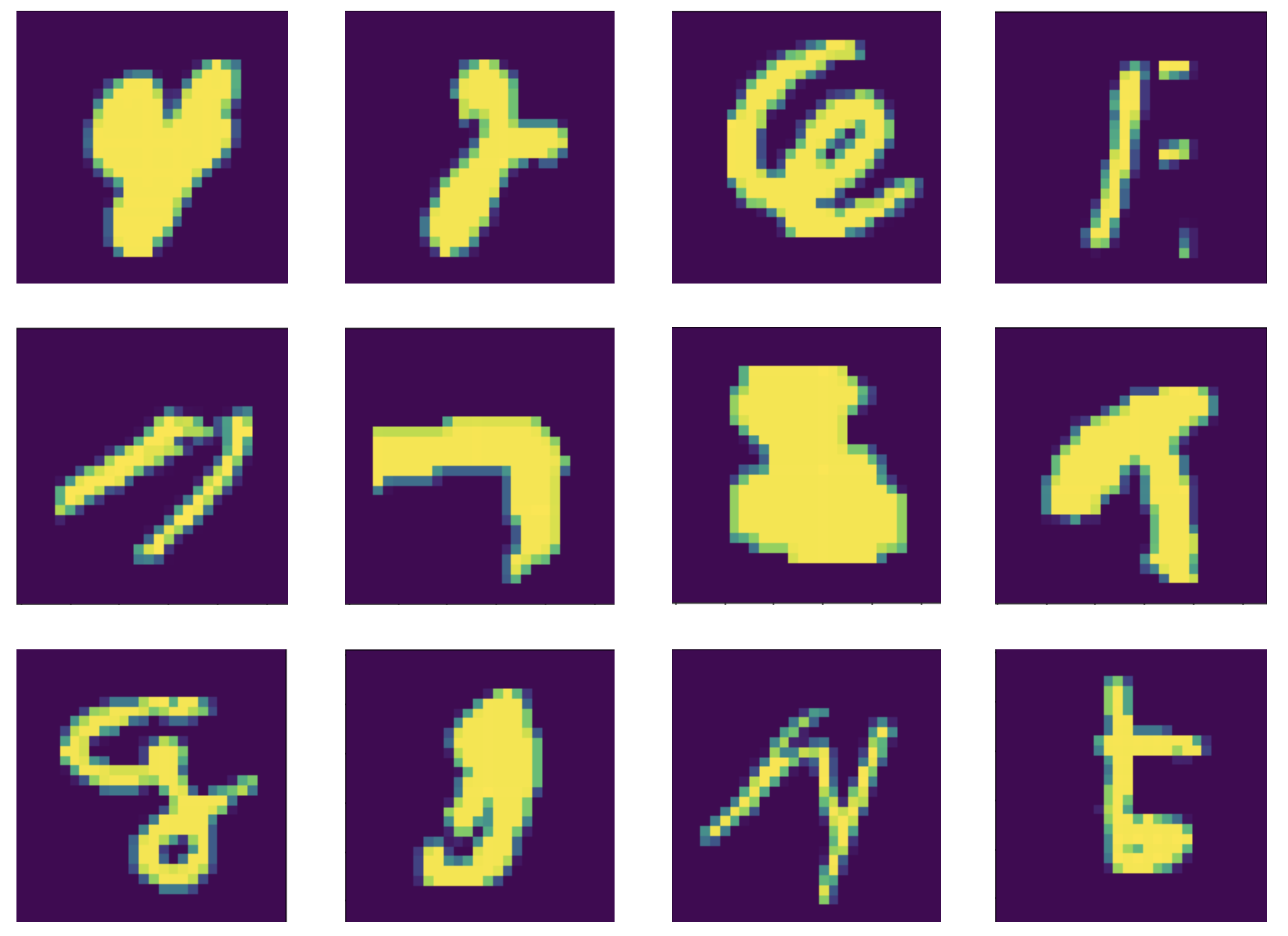
What are these? We don’t know either. But they’re all part of the MNIST training set. What’s even worse, however, is having perfectly valid inputs that end up mislabeled, like those shown in figure 5.3.
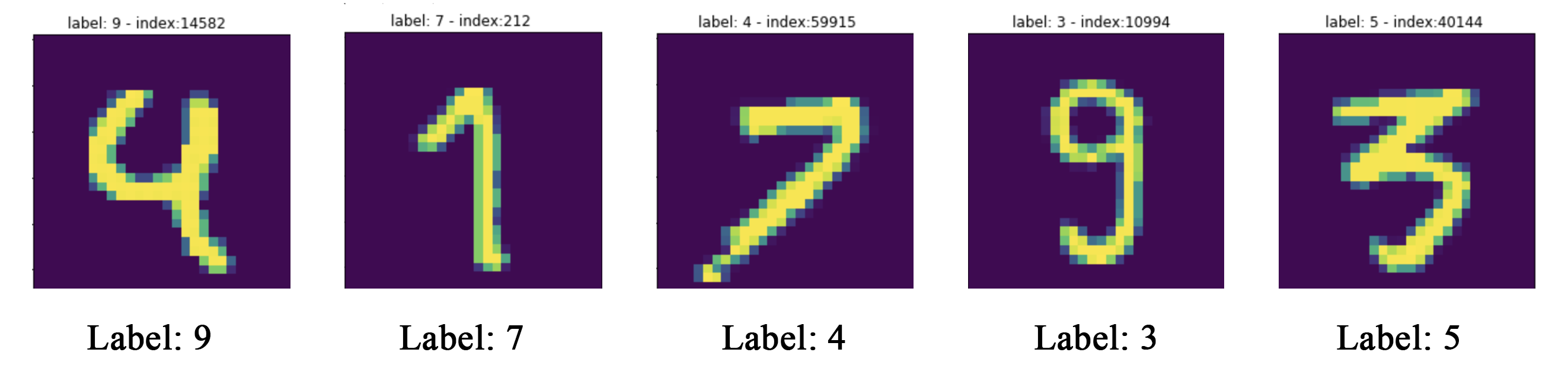
If a model goes out of its way to incorporate such outliers, its generalization performance will degrade, as shown in figure 5.4. For instance, a 4 that looks very close to the mislabeled 4 in figure 5.3 may end up getting classified as a 9.
5.1.1.2 Ambiguous features
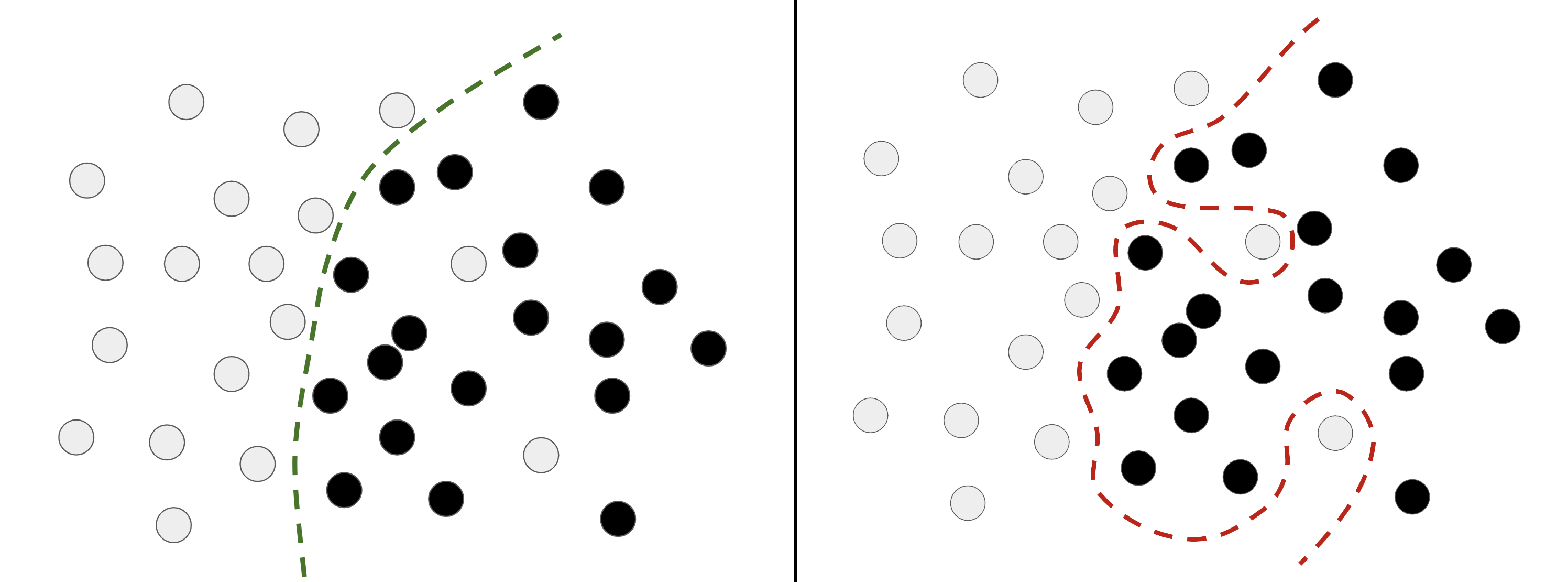
Not all data noise comes from inaccuracies—even perfectly clean and neatly labeled data can be noisy when the problem involves uncertainty and ambiguity (see figure 5.5). In classification tasks, it is often the case that some regions of the input feature space are associated with multiple classes at the same time. Let’s say we’re developing a model that takes an image of a banana and predicts whether the banana is unripened, ripe, or rotten. These categories have no objective boundaries, so the same picture might be classified as either unripened or ripe by different human labelers. Similarly, many problems involve randomness. We could use atmospheric pressure data to predict whether it will rain tomorrow, but the exact same measurements may be followed sometimes by rain and sometimes by a clear sky—with some probability.
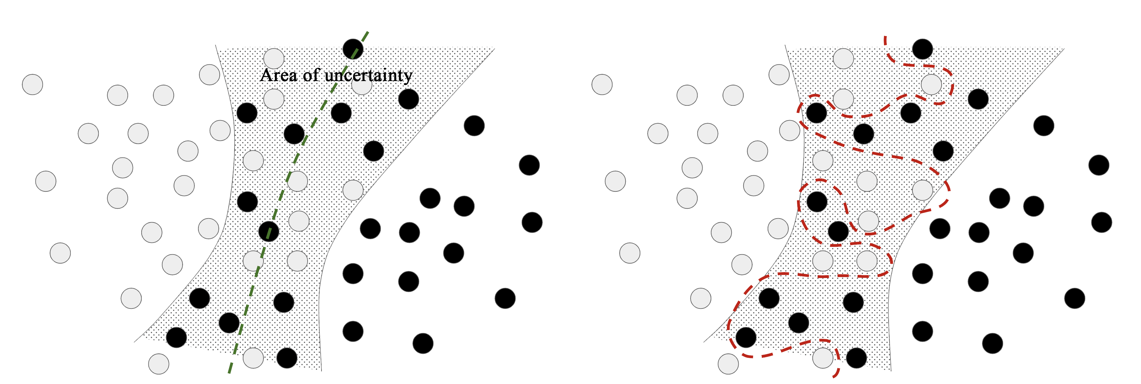
A model could overfit to such probabilistic data by being too confident about ambiguous regions of the feature space, as in figure 5.5. A more robust fit would ignore individual data points and look at the bigger picture.
5.1.1.3 Rare features and spurious correlations
If you’ve only ever seen two orange tabby cats in your life, and they both happened to be terribly antisocial, you might infer that orange tabby cats are generally likely to be antisocial. That’s overfitting: if you had been exposed to a wider variety of cats, including more orange ones, you’d have learned that cat color is not well correlated with character.
Likewise, machine learning models trained on datasets that include rare feature values are highly susceptible to overfitting. In a sentiment classification task, if the word cherimoya (a fruit native to the Andes) appears in only one text in the training data, and this text happens to be negative in sentiment, a poorly regularized model might put a very high weight on this word and always classify new texts that mention cherimoyas as negative. But objectively, there’s nothing negative about the cherimoya (Mark Twain called it “the most delicious fruit known to men”).
Importantly, a feature value doesn’t need to occur only a couple of times to lead to spurious correlations. Consider a word that occurs in 100 samples in your training data and that’s associated with a positive sentiment 54% of the time and with a negative sentiment 46% of the time. That difference may be a complete statistical fluke, yet your model is likely to learn to use that feature for its classification task. This is one of the most common sources of overfitting.
Here’s a striking example. Take MNIST. Create a new training set by concatenating 784 white-noise dimensions to the existing 784 dimensions of the data—so half of the data is now noise. For comparison, also create an equivalent dataset by concatenating 784 all-zero dimensions. Our concatenation of meaningless features does not affect the information content of the data at all: we’re only adding irrelevant data points. Human classification accuracy wouldn’t be affected by these transformations.
Now, let’s train the model from chapter 2 on both of these training sets.
get_model <- function() {
  model <- keras_model_sequential() |>
    layer_dense(512, activation = "relu") |>
    layer_dense(10, activation = "softmax")

  model |> compile(
    optimizer = "adam",
    loss = "sparse_categorical_crossentropy",
    metrics = c("accuracy")
  )

  model
}

model <- get_model()
history_noise <- model |> fit(
  train_images_with_noise_channels, train_labels,
  epochs = 10,
  batch_size = 128,
  validation_split = 0.2
)

model <- get_model()
history_zeros <- model |> fit(
  train_images_with_zeros_channels, train_labels,
  epochs = 10,
  batch_size = 128,
  validation_split = 0.2
)
Despite the data holding the same information in both cases, the validation accuracy of the model trained with noise channels ends up about one percentage point lower—purely through the influence of spurious correlations (figure 5.6). The more noise channels we add, the more the accuracy will degrade.
plot(NULL,
     main = "Effect of Noise Channels on Validation Accuracy",
     xlab = "Epochs", xlim = c(1, history_noise$params$epochs),
     ylab = "Validation Accuracy", ylim = c(0.9, 0.98), las = 1)
lines(history_zeros$metrics$val_accuracy, lty = 1, type = "o")
lines(history_noise$metrics$val_accuracy, lty = 2, type = "o")
legend("bottomright", lty = 1:2,
       legend = c("Validation accuracy with zeros channels",
                  "Validation accuracy with noise channels"))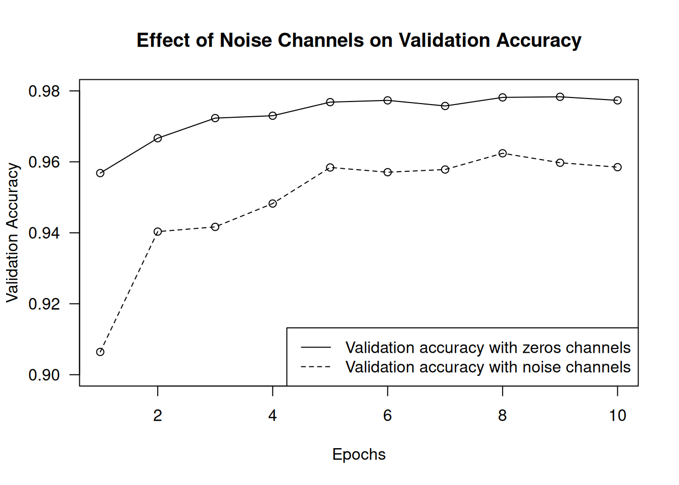
Noisy features inevitably lead to overfitting. As such, in cases where we aren’t sure whether the features we have are informative or distracting, it’s common to do feature selection before training. Restricting the IMDb data to the top 10,000 most common words is a crude form of feature selection, for instance. The typical way to do feature selection is to compute a usefulness score for each feature available—a measure of how informative the feature is with respect to the task, such as the mutual information between the feature and the labels—and keep only features that are above some threshold. Doing this would filter out the white-noise channels in the previous example.
5.1.2 The nature of generalization in deep learning
A remarkable fact about deep learning models is that they can be trained to fit anything, as long as they have enough representational power. Don’t believe us? Try shuffling the order of the MNIST labels, and then train a model. Even though there is no relationship whatsoever between the inputs and the shuffled labels, the training loss goes down just fine, even with a relatively small model. Naturally, the validation loss does not improve at all over time, because there is no possibility of generalization in this setting.
.[.[train_images, train_labels], .] <- dataset_mnist()
train_images <- array_reshape(train_images / 255,
                              c(60000, 28 * 28))

1random_train_labels <- sample(train_labels)

model <- keras_model_sequential() |>
  layer_dense(512, activation = "relu") |>
  layer_dense(10, activation = "softmax")

model |> compile(optimizer = "rmsprop",
                 loss = "sparse_categorical_crossentropy",
                 metrics = "accuracy")

history <- model |> fit(
  train_images, random_train_labels,
  epochs = 100, batch_size = 128,
  validation_split = 0.2
)- 1
- Shuffles the labels
In fact, we don’t even need to do this with MNIST data—we could just generate white-noise inputs and random labels. We could fit a model on that, too, as long as it has enough parameters. It would end up memorizing specific inputs like a lookup table.
If this is the case, then why do deep learning models generalize at all? Shouldn’t they just learn an ad hoc mapping between training inputs and targets, like a fancy hashtab() or dict()? What expectation can we have that this mapping will work for new inputs?
As it turns out, the nature of generalization in deep learning has little to do with deep learning models themselves and much to do with the structure of information in the real world. Let’s take a look at what’s really going on here.
5.1.2.1 The manifold hypothesis
The input to an MNIST classifier (before preprocessing) is a 28 × 28 array of integers between 0 and 255. The total number of possible input values is thus 256 to the power of 784—much greater than the number of atoms in the universe. However, very few of these inputs would look like valid MNIST samples: actual handwritten digits occupy only a tiny subspace of the parent space of all possible 28 × 28 arrays. What’s more, this subspace isn’t just a set of points sprinkled at random in the parent space: it is highly structured.
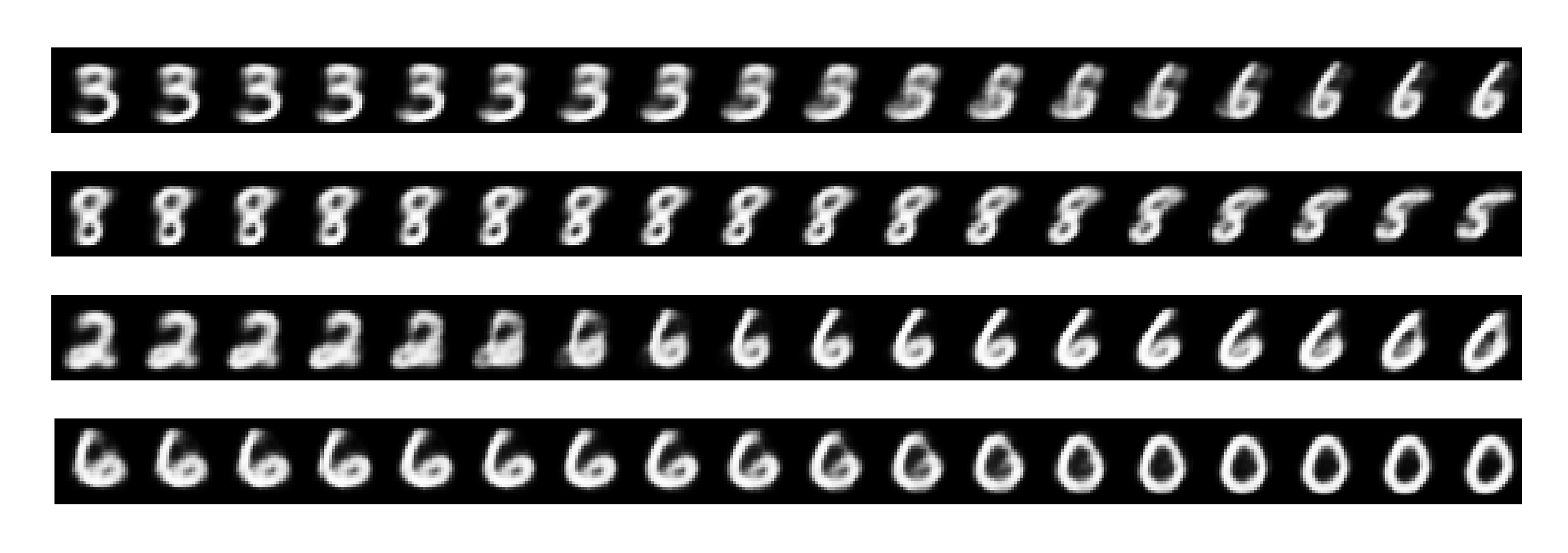
First, the subspace of valid handwritten digits is continuous: if we take a sample and modify it a little, it will still be recognizable as the same handwritten digit. Further, all samples in the valid subspace are connected by smooth paths that run through the subspace. This means that if we take two random MNIST digits A and B, there exists a sequence of “intermediate” images that morph A into B, such that two consecutive digits are very close to each other (see figure 5.7). There might be a few ambiguous shapes close to the boundary between two classes, but even these shapes would still look very digit-like.
In technical terms, we say that handwritten digits form a manifold within the space of possible 28 × 28 arrays. That’s a big word, but the concept is fairly intuitive. A manifold is a lower-dimensional subspace of some parent space that is locally similar to a linear (Euclidean) space. For instance, a smooth curve in the plane is a 1D manifold within a 2D space because for every point of the curve, we can draw a tangent (the curve can be approximated by a line at every point). A smooth surface within a 3D space is a 2D manifold, and so on.
More generally, the manifold hypothesis posits that all natural data lies on a low-dimensional manifold within the high-dimensional space where it is encoded. That’s a pretty strong statement about the structure of information in the universe. As far as we know, it’s accurate, and it’s the reason deep learning works. It’s true for MNIST digits, as well as for human faces, tree morphology, the sounds of the human voice, and even natural language.
The manifold hypothesis implies the following:
- Machine learning models only have to fit relatively simple, low-dimensional, highly structured subspaces within their potential input space (latent manifolds).
- Within one of these manifolds, it’s always possible to interpolate between two inputs—that is, morph one into another via a continuous path along which all points fall on the manifold.
The ability to interpolate between samples is the key to understanding generalization in deep learning.
5.1.2.2 Interpolation as a source of generalization
If we work with data points that can be interpolated, we can start making sense of points we’ve never seen before by relating them to other points that lie close on the manifold. In other words, we can make sense of the totality of the space using only a sample of the space. We can use interpolation to fill in the blanks.
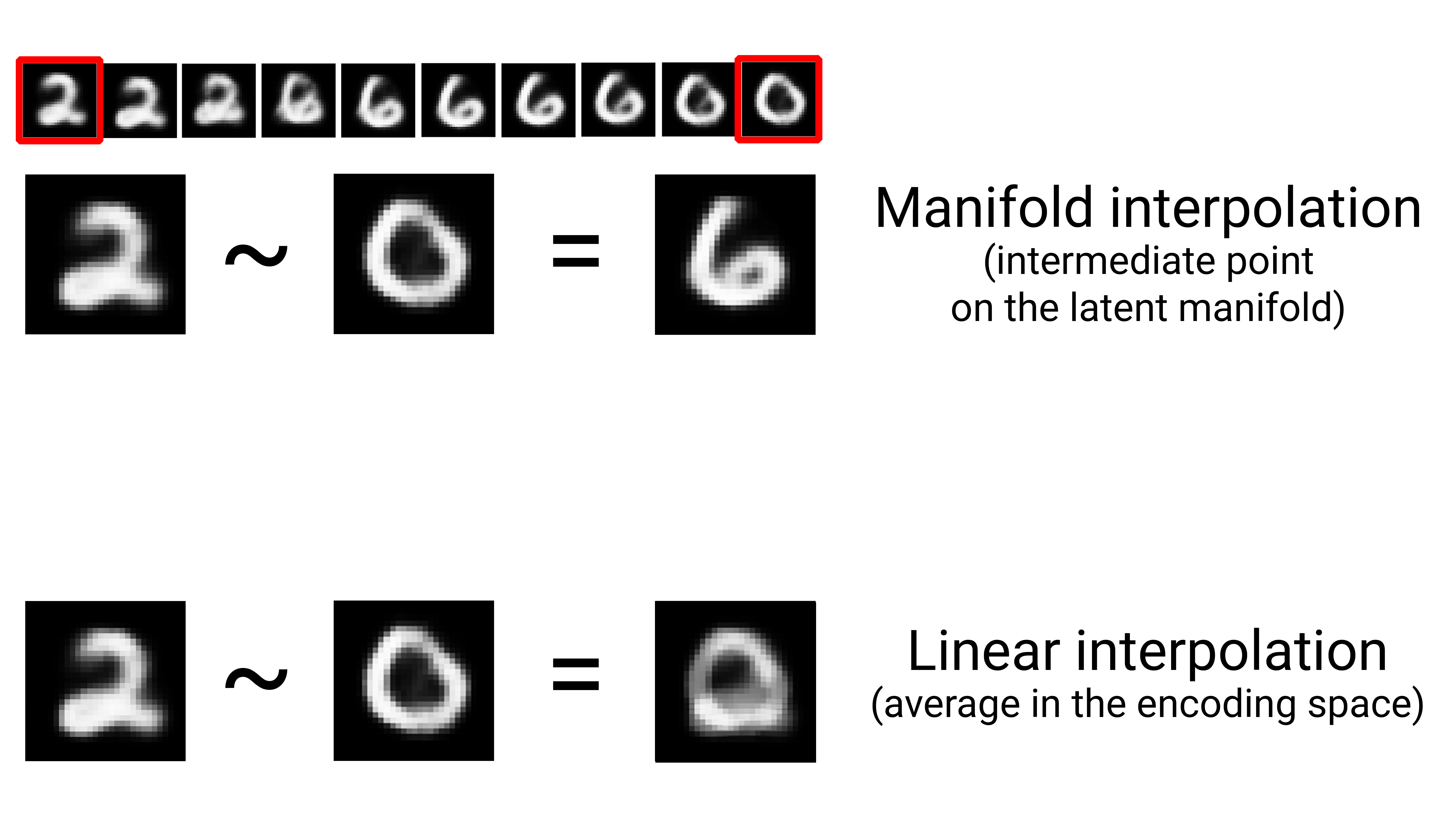
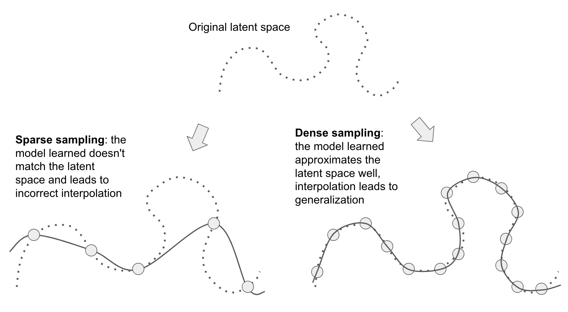
Note that interpolation on the latent manifold is different from linear interpolation in the parent space, as illustrated in figure 5.8. For instance, the average of pixels between two MNIST digits is usually not a valid digit.
Crucially, although deep learning achieves generalization via interpolation on a learned approximation of the data manifold, it would be a mistake to assume that interpolation is all there is to generalization. It’s the tip of the iceberg. Interpolation can only help you make sense of things that are very close to what you’ve seen before: it enables local generalization. But remarkably, humans deal with extreme novelty all the time, and they do just fine. You don’t need to be trained in advance on countless examples of every situation you’ll ever have to encounter. Every single one of your days is different from any day you’ve experienced before, and different from any day experienced by anyone since the dawn of humanity. You can switch between spending a week in NYC, a week in Shanghai, and a week in Bangalore without requiring thousands of lifetimes of learning and rehearsal for each city.
Humans are capable of extreme generalization, which is enabled by cognitive mechanisms other than interpolation: abstraction, symbolic models of the world, reasoning, logic, common sense, and innate priors about the world. This is what we generally call reason, as opposed to intuition and pattern recognition. The latter are largely interpolative in nature, but the former isn’t. Both are essential to intelligence. We’ll talk more about this in chapter 19.
5.1.2.3 Why deep learning works
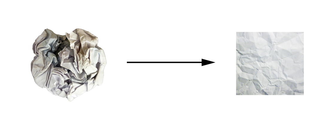
Remember the crumpled paper ball metaphor from chapter 2? A sheet of paper represents a 2D manifold within 3D space (figure 5.9). A deep learning model is a tool for uncrumpling paper balls—that is, for disentangling latent manifolds.
A deep learning model is basically a very high-dimensional curve. The curve is smooth and continuous (with additional constraints on its structure, originating from model architecture priors) because it needs to be differentiable. And that curve is fitted to data points via gradient descent—smoothly and incrementally. By construction, deep learning is about taking a big, complex curve—a manifold—and incrementally adjusting its parameters until it fits some training data points.
The curve involves enough parameters that it could fit anything. Indeed, if we let our model train for long enough, it will effectively end up purely memorizing its training data and won’t generalize at all. However, the data we’re fitting to isn’t made of isolated points sparsely distributed across the underlying space. Our data forms a highly structured, low-dimensional manifold within the input space—that’s the manifold hypothesis. And because fitting our model curve to this data happens gradually and smoothly over time, as gradient descent progresses, there will be an intermediate point during training at which the model roughly approximates the natural manifold of the data, as you can see in figure 5.10.
Moving along the curve learned by the model at that point will come close to moving along the actual latent manifold of the data. As such, the model will be capable of making sense of never-before-seen inputs via interpolation between training inputs.
Besides the trivial fact that they have sufficient representational power, there are a few properties of deep learning models that make them particularly well-suited to learning latent manifolds:
- Deep learning models implement a smooth, continuous mapping from their inputs to their outputs. It has to be smooth and continuous because it must be differentiable, by necessity (we couldn’t do gradient descent otherwise). This smoothness helps approximate latent manifolds, which follow the same properties.
- Deep learning models tend to be structured in a way that mirrors the “shape” of the information in their training data (via architecture priors). This is the case in particular for image-processing models (see chapters 8–12) and sequence-processing models (see chapter 13). More generally, deep neural networks structure their learned representations in a hierarchical and modular way, which echoes the way natural data is organized.
5.1.2.4 Training data is paramount
Although deep learning is indeed well-suited to manifold learning, the power to generalize is more a consequence of the natural structure of our data than a consequence of any property of our model. We’ll only be able to generalize if our data forms a manifold where points can be interpolated. The more informative and the less noisy our features are, the better we will be able to generalize, because our input space will be simpler and better structured. Data curation and feature engineering are essential to generalization.
Further, because deep learning is curve-fitting, for a model to perform well, it needs to be trained on a dense sampling of its input space. A dense sampling in this context means that the training data should densely cover the entirety of the input data manifold (see figure 5.11). This is especially true near decision boundaries. With a sufficiently dense sampling, it becomes possible to make sense of new inputs by interpolating between past training inputs, without having to use common-sense, abstract reasoning, or external knowledge about the world—all things that machine learning models have no access to.
As such, you should always keep in mind that the best way to improve a deep learning model is to train it on more data or better data (of course, adding overly noisy or inaccurate data will harm generalization). A denser coverage of the input data manifold will yield a model that generalizes better. You should never expect a deep learning model to perform anything more than crude interpolation between its training samples, and thus, you should do everything you can to make interpolation as easy as possible. The only thing you will find in a deep learning model is what you put into it: the priors encoded in its architecture and the data it was trained on.
When getting more data isn’t possible, the next-best solution is to modulate the quantity of information a model is allowed to store or to add constraints on the smoothness of the model curve. If a network can afford to memorize only a small number of patterns, or very regular patterns, the optimization process will force it to focus on the most prominent patterns, which have a better chance of generalizing well. The process of fighting overfitting this way is called regularization. We’ll review regularization techniques in depth in section 5.4.4.
Before we can start tweaking our model to help it generalize better, we need a way to assess how our model is currently doing. In the following section, you’ll learn about how you can monitor generalization during model development: model evaluation.
5.2 Evaluating machine learning models
We can only control what we can observe. Because our goal is to develop models that can successfully generalize to new data, it’s essential to be able to reliably measure the generalization power of our model. In this section, we’ll formally introduce the different ways we can evaluate machine learning models. You already saw most of them in action in the previous chapter.
5.2.1 Training, validation, and test sets
Evaluating a model always boils down to splitting the available data into three sets: training, validation, and test. We train on the training data and evaluate our model on the validation data. Once our model is ready for prime time, we test it one final time on the test data, which is meant to be as similar as possible to production data. Then we can deploy the model in production.
You may ask, why not have two sets: a training set and a test set? You’d train on the training data and evaluate on the test data. Much simpler!
The reason is that developing a model always involves tuning its configuration: for example, choosing the number of layers or the size of the layers (called the hyperparameters of the model, to distinguish them from the parameters, which are the network’s weights). We do this tuning by using as a feedback signal the performance of the model on the validation data. In essence, this tuning is a form of learning: a search for a good configuration in some parameter space. As a result, tuning the configuration of the model based on its performance on the validation set can quickly result in overfitting to the validation set, even though our model is never directly trained on it.
Central to this phenomenon is the notion of information leaks. Every time we tune a hyperparameter of our model based on the model’s performance on the validation set, some information about the validation data leaks into the model. If we do this only once, for one parameter, then very few bits of information will leak, and our validation set will remain reliable to evaluate the model. But if we repeat this many times—running one experiment, evaluating on the validation set, and modifying our model as a result—then we’ll leak an increasingly significant amount of information about the validation set into the model.
At the end of the day, we’ll end up with a model that performs artificially well on the validation data because that’s what we optimized it for. We care about performance on completely new data, not the validation data, so we need to use a completely different, never-before-seen dataset to evaluate the model: the test dataset. Our model shouldn’t have had access to any information about the test set, even indirectly. If anything about the model has been tuned based on test set performance, then our measure of generalization will be flawed.
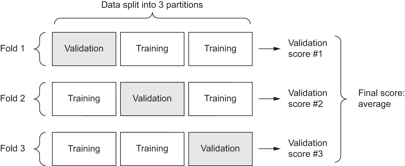
Splitting our data into training, validation, and test sets may seem straightforward, but there are a few advanced ways to do it that can come in handy when little data is available. Let’s review three classic evaluation recipes: simple hold-out validation, K-fold validation, and iterated K-fold validation with shuffling. We’ll also talk about the use of common-sense baselines to check that our training is going somewhere.
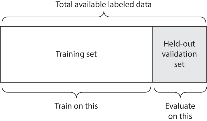
5.2.1.1 Simple hold-out validation
Set apart some fraction of your data as your test set. Train on the remaining data, and evaluate on the test set. As you saw in the previous sections, to prevent information leaks, you shouldn’t tune your model based on the test set, and therefore you should also reserve a validation set.
Schematically, hold-out validation looks like figure 5.12. The following listing shows a simple implementation.
num_validation_samples <- 10000
1val_indices <- sample.int(nrow(data), num_validation_samples)
2validation_data <- data[val_indices, ]
3training_data <- data[-val_indices, ]
4model <- get_model()
fit(model, training_data, ...)
validation_score <- evaluate(model, validation_data, ...)

5...

6model <- get_model()
fit(model, data, ...)
test_score <- evaluate(model, test_data, ...)- 1
- Shuffling the data is usually appropriate.
- 2
- Defines the validation set
- 3
- Defines the training set
- 4
- Trains a model on the training data, and evaluates it on the validation data
- 5
- At this point, we can tune our model, retrain it, evaluate it, tune it again…
- 6
- Once we’ve tuned our hyperparameters, it’s common to train our final model from scratch on all non-test data available.
This is the simplest evaluation protocol, and it suffers from one flaw: if little data is available, then our validation and test sets may contain too few samples to be statistically representative of the data at hand. This is easy to recognize: if different random shuffling rounds of the data before splitting end up yielding very different measures of model performance, then you’re having this problem. K-fold validation and iterated K‑fold validation are two ways to address this, as discussed next.
5.2.1.2 K-fold validation
With this approach, we split our data into K partitions of equal size. For each partition i, train a model on the remaining K – 1 partitions and evaluate it on partition i. The final score is then the average of the K scores obtained. This method is helpful when the performance of our model shows significant variance based on our train-test split. Like hold-out validation, this method doesn’t exempt us from using a distinct validation set for model calibration.
Schematically, K-fold cross-validation looks like figure 5.13. The next listing shows a simple implementation.
k <- 3
fold_id <- sample(rep(1:k, length.out = nrow(data)))
validation_scores <- numeric(k)

for (fold in seq_len(k)) {
1  validation_idx <- which(fold_id == fold)

  validation_data <- data[validation_idx, ]
2  training_data <- data[-validation_idx, ]
3  model <- get_model()
  fit(model, training_data, ...)
  validation_score <- evaluate(model, validation_data, ...)
  validation_scores[[fold]] <- validation_score
}

4validation_score <- mean(validation_scores)
5model <- get_model()
fit(model, data, ...)
test_score <- evaluate(model, test_data, ...)- 1
- Selects the validation-data partition
- 2
- Uses the remainder of the data as training data
- 3
- Creates a brand-new instance of the model (untrained)
- 4
- Validation score: average of the validation scores of the k folds
- 5
- Trains the final model on all non-test data available
5.2.1.3 Iterated K-fold validation with shuffling
This one is for situations in which we have relatively little data available and we need to evaluate our model as precisely as possible. We’ve found it to be extremely helpful in Kaggle competitions. It consists of applying K-fold validation multiple times, shuffling the data every time before splitting it K ways. The final score is the average of the scores obtained at each run of K-fold validation. Note that we end up training and evaluating P × K models (where P is the number of iterations we use), which can be very expensive.
5.2.2 Beating a common-sense baseline
Besides the different evaluation protocols available, you should also know about using common-sense baselines. Training a deep learning model is a bit like pressing a button that launches a rocket in a parallel world. We can’t hear it or see it. We can’t observe the manifold learning process—it’s happening in a space with thousands of dimensions, and even if we projected it to 3D, we couldn’t interpret it. The only feedback we have is our validation metrics—like an altitude meter on our invisible rocket. A particularly important point is to be able to tell whether we’re getting off the ground at all. What was the altitude we started at? Our model seems to have an accuracy of 15%; is that any good?
Before you start working with a dataset, you should always pick a trivial baseline that you’ll try to beat. If you cross that threshold, you’ll know you’re doing something right: your model is actually using the information in the input data to make predictions that generalize—you can keep going. This baseline could be the performance of a random classifier or the performance of the simplest non-machine learning technique you can imagine.
For instance, in the MNIST digit-classification example, a simple baseline would be a validation accuracy greater than 0.1 (random classifier); in the IMDb example, it would be a validation accuracy greater than 0.5. In the Reuters example, it would be around 0.18–0.19, due to class imbalance. If you have a binary classification problem where 90% of samples belong to class A and 10% belong to class B, then a classifier that always predicts A already achieves 0.9 in validation accuracy, and you’ll need to do better than that.
Having a common-sense baseline to refer to is essential when you’re getting started on a problem no one has solved before. If you can’t beat a trivial solution, your model is worthless—perhaps you’re using the wrong model, or perhaps the problem you’re tackling can’t even be approached with machine learning in the first place. Time to go back to the drawing board.
5.2.3 Things to keep in mind about model evaluation
Keep an eye out for the following when you’re choosing an evaluation protocol:
- Data representativeness—You want both your training set and test set to be representative of the data at hand. For instance, if you’re trying to classify images of digits, and you’re starting from an array of samples where the samples are ordered by their class, taking the first 80% of the array as your training set and the remaining 20% as your test set will result in your training set containing only classes 0–7, whereas your test set contains only classes 8–9. This seems like a ridiculous mistake, but it’s surprisingly common. For this reason, you usually should randomly shuffle your data before splitting it into training and test sets.
- The arrow of time—If you’re trying to predict the future given the past (for example, tomorrow’s weather, stock movements, and so on), you should not randomly shuffle your data before splitting it because doing so will create a temporal leak: your model will effectively be trained on data from the future. In such situations, you should always make sure the data in your test set is posterior to the data in the training set.
- Redundancy in your data—If some data points in your data appear twice (fairly common with real-world data), then shuffling the data and splitting it into a training set and a validation set will result in redundancy between the training and validation sets. In effect, you’ll be testing on part of your training data, which is the worst thing you can do! Make sure your training set and validation set are disjoint.
Having a reliable way to evaluate the performance of your model is how you’ll be able to monitor the tension at the heart of machine learning—between optimization and generalization, underfitting and overfitting.
5.3 Improving model fit
To achieve the perfect fit, we must first overfit. Because we don’t know in advance where the boundary lies, we must cross it to find it. Thus, our initial goal as we start working on a problem is to achieve a model that shows some generalization power and that is able to overfit. Once we have such a model, we’ll focus on refining generalization by fighting overfitting.
Three common problems occur at this stage:
- Training doesn’t get started: the training loss doesn’t go down over time.
- Training gets started just fine, but the model doesn’t meaningfully generalize: we can’t beat the common-sense baseline we set.
- Training and validation loss both go down over time, and we can beat the baseline, but we don’t seem to be able to overfit, which indicates we’re still underfitting.
Let’s see how to address these problems to achieve the first big milestone of a machine learning project: getting a model that has some generalization power (it can beat a trivial baseline) and is able to overfit.
5.3.1 Tuning key gradient descent parameters
Sometimes, training doesn’t get started or stalls too early. The loss is stuck. This is always something you can overcome: remember that you can fit a model to random data. Even if nothing about your problem makes sense, you should still be able to train something—if only by memorizing the training data.
When this happens, it’s always a problem with the configuration of the gradient descent process: your choice of optimizer, the distribution of initial values in the weights of your model, your learning rate, or your batch size. All these parameters are interdependent, and as such, it is usually sufficient to tune the learning rate and the batch size while maintaining the rest of the parameters constant.
Let’s look at a concrete example. We’ll train the MNIST model from chapter 2 with an inappropriately large learning rate, of value 1.
.[.[train_images, train_labels], .] <- dataset_mnist()
train_images <- array_reshape(train_images / 255,
                              c(60000, 28 * 28))

model <- keras_model_sequential() |>
  layer_dense(512, activation = "relu") |>
  layer_dense(10, activation = "softmax")

model |> compile(
  optimizer = optimizer_rmsprop(1),
  loss = "sparse_categorical_crossentropy",
  metrics = "accuracy"
)

history <- model |> fit(
  train_images, train_labels,
  epochs = 10, batch_size = 128,
  validation_split = 0.2
)
The model quickly reaches a training and validation accuracy in the 20% to 40% range, but it cannot get past that. Let’s try to lower the learning rate to a more reasonable value of 1e-2.
model <- keras_model_sequential() |>
  layer_dense(512, activation = "relu") |>
  layer_dense(10, activation = "softmax")

model |> compile(
  optimizer = optimizer_rmsprop(1e-2),
  loss = "sparse_categorical_crossentropy",
  metrics = "accuracy"
)

history <- model |> fit(
  train_images, train_labels,
  epochs = 10, batch_size = 128,
  validation_split = 0.2
)
The model is now able to train.
If you find yourself in a similar situation, try one of the following:
- Lower or increase the learning rate. A learning rate that is too high may lead to updates that vastly overshoot a proper fit, as in the previous example; and a learning rate that is too low may make training so slow that it appears to stall.
- Increase the batch size. A batch with more samples will lead to gradients that are more informative and less noisy (lower variance).
Eventually, you’ll find a configuration that gets training started.
5.3.2 Using better architecture priors
You have a model that fits, but for some reason, your validation metrics aren’t improving. They remain no better than what a random classifier would achieve: your model trains but doesn’t generalize. What’s going on?
This is perhaps the worst machine learning situation you can find yourself in. It indicates that something is fundamentally wrong with your approach, and it may not be easy to tell what. Here are some tips.
First, the input data you’re using simply may not contain sufficient information to predict your targets: the problem as formulated is not solvable. This is what happened earlier when we tried to fit an MNIST model in which the labels were shuffled: the model trained just fine, but validation accuracy stayed stuck at 10% because it was plainly impossible to generalize with such a dataset.
The kind of model you’re using also may not be suited to the problem at hand. For instance, in chapter 13, you’ll see an example of a timeseries prediction problem in which a densely connected architecture can’t beat a trivial baseline, whereas a more appropriate recurrent architecture does manage to generalize well. Using a model that makes the right assumptions about the problem is essential to achieve generalization: you should use the right architecture priors.
In the following chapters, you’ll learn about the best architectures to use for a variety of data modalities: images, text, timeseries, and so on. In general, you should always be sure to read up on architecture best practices for the kind of task you’re attacking—chances are, you’re not the first person to attempt it.
5.3.3 Increasing model capacity
If you manage to get to a model that fits, with validation metrics going down, and the model seems to achieve at least some level of generalization power, congratulations: you’re almost there. Next, you need to get your model to start overfitting.
Consider the following small model: a simple logistic regression trained on MNIST pixels.
model <- keras_model_sequential() |>
  layer_dense(10, activation = "softmax")

model |> compile(
  optimizer = "rmsprop",
  loss = "sparse_categorical_crossentropy",
  metrics = "accuracy"
)

history_small_model <- model |> fit(
  train_images, train_labels,
  epochs = 20,
  batch_size = 128,
  validation_split = 0.2
)
We get the loss curves shown in figure 5.14.
plot(history_small_model$metrics$val_loss, type = 'o',
     main = "Effect of Insufficient Model Capacity on Validation Loss",
     xlab = "Epochs", ylab = "Validation Loss")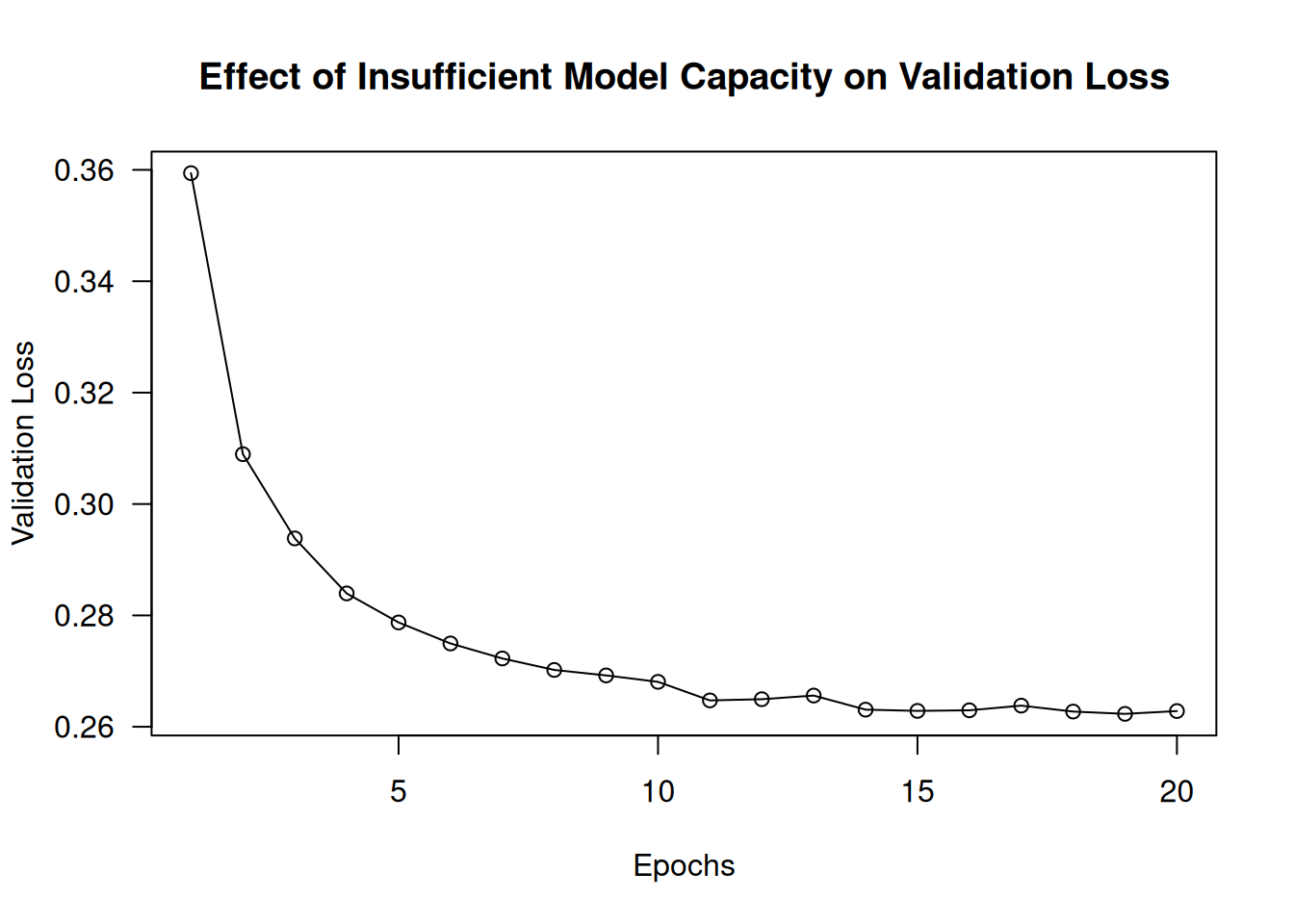
The validation metrics seem to stall or to improve very slowly, instead of peaking and reversing course. The validation loss goes to 0.26 and stays there. We can fit, but we can’t overfit, even after many iterations over the training data. You’re likely to encounter similar curves often in your career.
Remember that it should always be possible to overfit. Much like the problem “The training loss doesn’t go down,” this is a problem that can always be solved. If you don’t seem able to overfit, it’s likely a problem with the representational power of your model. You’re going to need a bigger model: one with more capacity—that is, able to store more information. You can increase representational power by adding more layers, using bigger layers (layers with more parameters), or using kinds of layers that are more appropriate for the problem at hand (better architecture priors).
Let’s try training a bigger model, with 2 intermediate layers that have 128 units each:
model <- keras_model_sequential() |>
    layer_dense(128, activation="relu") |>
    layer_dense(128, activation="relu") |>
    layer_dense(10, activation="softmax")

model |> compile(
  optimizer="rmsprop",
  loss="sparse_categorical_crossentropy",
  metrics="accuracy"
)

history_large_model <- model |> fit(
  train_images, train_labels,
  epochs = 20,
  batch_size = 128,
  validation_split = 0.2
)
The training curves now look exactly like they should: the model fits fast and starts overfitting after eight epochs (see figure 5.15):
plot(history_large_model$metrics$val_loss, type = 'o',
     main = "Validation Loss for a Model with Appropriate Capacity",
     xlab = "Epochs", ylab = "Validation Loss")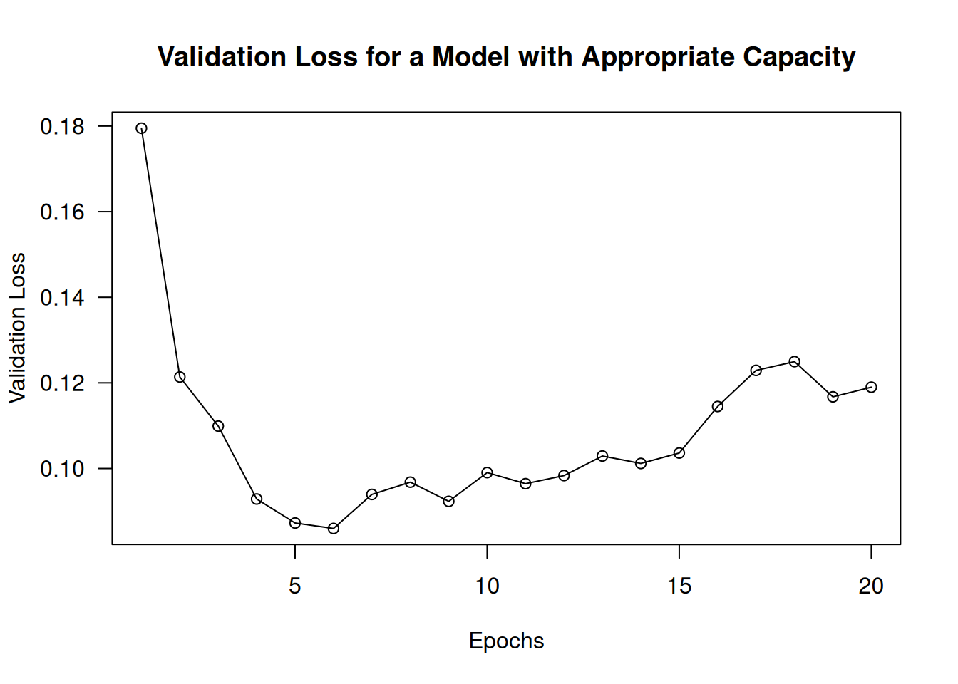
Note that although it is standard to work with models that are way over-parameterized for the problem at hand, there can definitely be such a thing as too much memorization capacity. You’ll know your model is too large if it starts overfitting right away. Here’s what happens for an MNIST model with 3 intermediate layers that have 2,048 units each (see figure 5.16):
model <- keras_model_sequential() |>
  layer_dense(2048, activation = "relu") |>
  layer_dense(2048, activation = "relu") |>
  layer_dense(2048, activation = "relu") |>
  layer_dense(10, activation = "softmax")

model |> compile(
  optimizer = "rmsprop",
  loss = "sparse_categorical_crossentropy",
  metrics = "accuracy"
)

history_very_large_model <- model |> fit(
  train_images, train_labels,
  epochs = 20,
1  batch_size = 32,
  validation_split = 0.2
)- 1
- When training larger models, we can reduce the batch size to limit memory consumption.
plot(history_very_large_model$metrics$val_loss, type = 'o',
     main = "Validation Loss for a Model with Too Much Capacity",
     xlab = "Epochs", ylab = "Validation Loss")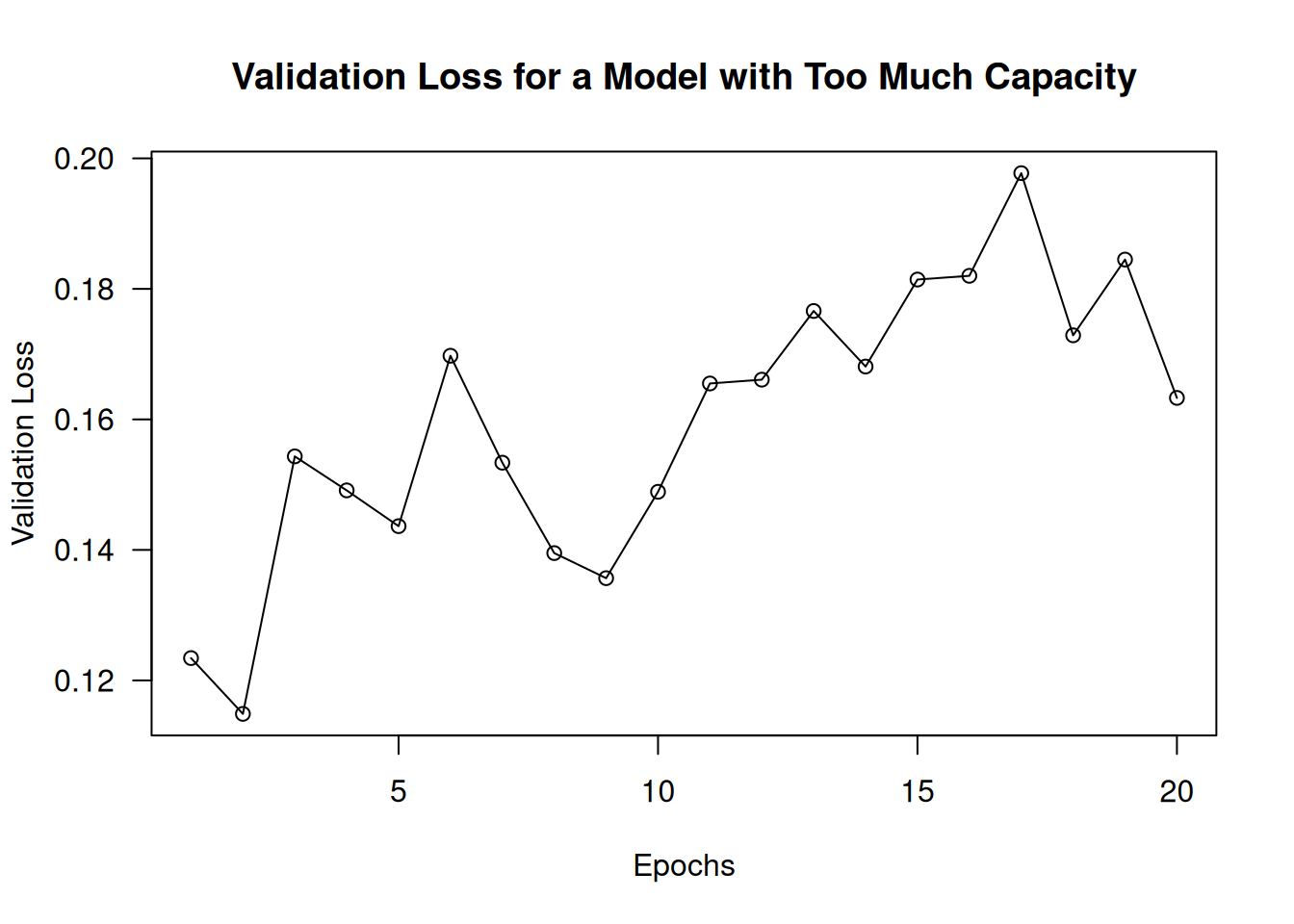
5.4 Improving generalization
Once our model has demonstrated some generalization power and the ability to overfit, it’s time to switch our focus to maximizing generalization.
5.4.1 Dataset curation
You’ve already learned that generalization in deep learning originates from the latent structure of your data. If your data makes it possible to smoothly interpolate between samples, then you will be able to train a deep learning model that generalizes. If your problem is overly noisy or fundamentally discrete—like, say, list sorting—then deep learning will not help you. Deep learning is curve-fitting, not magic.
As such, it is essential to be sure you’re working with an appropriate dataset. Spending more effort and money on data collection almost always yields a much greater return on investment than spending the same on developing a better model:
- Be sure you have enough data. Remember that you need a dense sampling of the input–output space. More data will yield a better model. Sometimes, problems that seem impossible at first become solvable with a larger dataset.
- Minimize labeling errors: visualize inputs to check for anomalies, and proofread your labels.
- Clean your data, and deal with missing values (we cover this in the next chapter).
- If you have many features and you aren’t sure which ones are actually useful, do feature selection.
A particularly important way you can improve the generalization potential of your data is feature engineering. For most machine learning problems, feature engineering is a key ingredient for success. Let’s take a look.
5.4.2 Feature engineering
Feature engineering is the process of using our own knowledge about the data and about the machine learning algorithm at hand (in this case, a neural network) to make the algorithm work better by applying hardcoded (non-learned) transformations to the data before it goes into the model. In many cases, it isn’t reasonable to expect a machine learning model to be able to learn from completely arbitrary data. The data needs to be presented to the model in a way that will make the model’s job easier.
Let’s look at an intuitive example. Suppose we’re trying to develop a model that can take as input an image of a clock and can output the time of day (see figure 5.17).
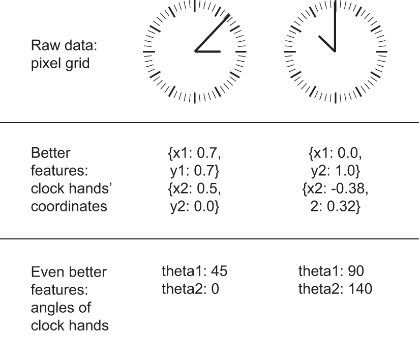
If we choose to use the raw pixels of the image as input data, then we have a difficult machine learning problem on our hands. We’ll need a convolutional neural network to solve it, and we’ll have to expend a lot of computational resources to train the network.
But if we already understand the problem at a high level (we understand how humans read time on a clock face), then we can come up with much better input features for a machine learning algorithm: for instance, it’s easy to write a five-line R script to follow the black pixels of the clock hands and output the (x, y) coordinates of the tip of each hand. Then a simple machine learning algorithm can learn to associate these coordinates with the appropriate time of day.
We can go even further: do a coordinate change and express the (x, y) coordinates as polar coordinates with regard to the center of the image. Our input will become the angle theta of each clock hand. At this point, our features make the problem so easy that no machine learning is required; a simple rounding operation and dictionary lookup are enough to recover the approximate time of day.
That’s the essence of feature engineering: making a problem easier by expressing it in a simpler way. Make the latent manifold smoother, simpler, and better organized. Doing so usually requires understanding the problem in depth.
Before deep learning, feature engineering used to be the most important part of the machine learning workflow because classical shallow algorithms didn’t have hypothesis spaces rich enough to learn useful features by themselves. The way we presented the data to the algorithm was absolutely critical to its success. For instance, before convolutional neural networks became successful on the MNIST digit-classification problem, solutions were typically based on hardcoded features such as the number of loops in a digit image, the height of each digit in an image, a histogram of pixel values, and so on.
Fortunately, modern deep learning removes the need for most feature engineering because neural networks are capable of automatically extracting useful features from raw data. Does this mean we don’t have to worry about feature engineering as long as we’re using deep neural networks? No, for two reasons:
- Good features still allow us to solve problems more elegantly while using fewer resources. For instance, it would be ridiculous to solve the problem of reading a clock face using a convolutional neural network.
- Good features let us solve a problem with far less data. The ability of deep learning models to learn features on their own relies on having lots of training data available; if we have only a few samples, then the information value in their features becomes critical.
5.4.3 Using early stopping
In deep learning, we always use models that are vastly over-parameterized: they have way more degrees of freedom than the minimum necessary to fit to the latent manifold of the data. This over-parameterization is not a problem because we never fully fit a deep learning model. Such a fit wouldn’t generalize at all. We will always interrupt training long before we’ve reached the minimum possible training loss. Finding the exact point during training where we’ve reached the most generalizable fit—the exact boundary between an underfit curve and an overfit curve—is one of the most effective things we can do to improve generalization.
In the examples from the previous chapter, we started by training our models for longer than necessary to figure out the number of epochs that yielded the best validation metrics; then we retrained a new model for exactly that number of epochs. This is pretty standard. However, it requires us to do redundant work, which can sometimes be expensive. Naturally, we could save our model at the end of each epoch and then, once we found the best epoch, reuse the closest saved model we had. In Keras, it’s typical to do this with the callback_early_stopping() callback, which interrupts training as soon as validation metrics have stopped improving, while remembering the best known model state. You’ll learn to use callbacks in chapter 7.
5.4.4 Regularizing a model
Regularization techniques are a set of best practices that actively impede the model’s ability to fit perfectly to the training data, with the goal of making the model perform better during validation. This is called regularizing the model because it tends to make the model simpler, more “regular,” with its curve smoother and more “generic”—and thus less specific to the training set and better able to generalize by more closely approximating the latent manifold of the data. Keep in mind that regularizing a model is a process that should always be guided by an accurate evaluation procedure. We will achieve generalization only if we can measure it. Let’s review some of the most common regularization techniques and apply them in practice to improve the movie classification model from chapter 4.
5.4.4.1 Reducing the network’s size
You’ve already learned that a model that is too small will not overfit. The simplest way to mitigate overfitting is to reduce the size of the model (the number of learnable parameters in the model, determined by the number of layers and the number of units per layer). If the model has limited memorization resources, it won’t be able to simply memorize its training data. To minimize its loss, it will have to resort to learning compressed representations that have predictive power regarding the targets—precisely the type of representations we’re interested in. At the same time, keep in mind that we should use models that have enough parameters that they don’t underfit: the model shouldn’t be starved for memorization resources. There is a compromise to be found between too much capacity and not enough capacity.
Unfortunately, there is no magical formula to determine the right number of layers or the right size for each layer. We must evaluate an array of different architectures (on our validation set, not on our test set, of course) to find the correct model size for our data. The general workflow to find an appropriate model size is to start with relatively few layers and parameters and increase the size of the layers or add new layers until we see diminishing returns with regard to validation loss.
Let’s try this on the movie-review classification model. Here’s a condensed version of the model from chapter 4.
.[.[train_data, train_labels], .] <- dataset_imdb(num_words = 10000)

vectorize_sequences <- function(sequences, dimension = 10000) {
  results <- matrix(0, nrow = length(sequences), ncol = dimension)
  for (i in seq_along(sequences)) {
    idx <- sequences[[i]] + 1L
    idx <- idx[idx <= dimension]
    results[i, idx] <- 1
  }
  results
}

train_data <- vectorize_sequences(train_data)

model <- keras_model_sequential() |>
    layer_dense(16, activation="relu") |>
    layer_dense(16, activation="relu") |>
    layer_dense(1, activation="sigmoid")

model |> compile(
  optimizer = "rmsprop",
  loss = "binary_crossentropy",
  metrics = "accuracy"
)

history_original <- model |> fit(
  train_data, train_labels,
  epochs = 20, batch_size = 512, validation_split = 0.4
)
Now, let’s try to replace it with this smaller model.
model <- keras_model_sequential() |>
  layer_dense(4, activation = "relu") |>
  layer_dense(4, activation = "relu") |>
  layer_dense(1, activation = "sigmoid")

model |> compile(
  optimizer = "rmsprop",
  loss = "binary_crossentropy",
  metrics = "accuracy"
)

history_smaller_model <- model |> fit(
  train_data, train_labels,
  epochs = 20, batch_size = 512, validation_split = 0.4
)
Figure 5.18 shows a comparison of the validation losses of the original model and the smaller model. As you can see, the smaller model starts overfitting later than the reference model (after six epochs rather than four), and its performance degrades more slowly once it starts overfitting.
plot(
  NULL,
  main = "Original Model vs. Smaller Model on IMDB Review Classification",
  xlab = "Epochs",
  xlim = c(1, history_original$params$epochs),
  ylab = "Validation Loss",
  ylim = extendrange(c(history_original$metrics$val_loss,
                       history_smaller_model$metrics$val_loss)),
  panel.first = abline(v = 1:history_original$params$epochs,
                       lty = "dotted", col = "lightgrey")
)

lines(history_original     $metrics$val_loss, lty = 2)
lines(history_smaller_model$metrics$val_loss, lty = 1)
legend("topleft", lty = 2:1,
       legend = c("Validation loss of original model",
                  "Validation loss of smaller model"))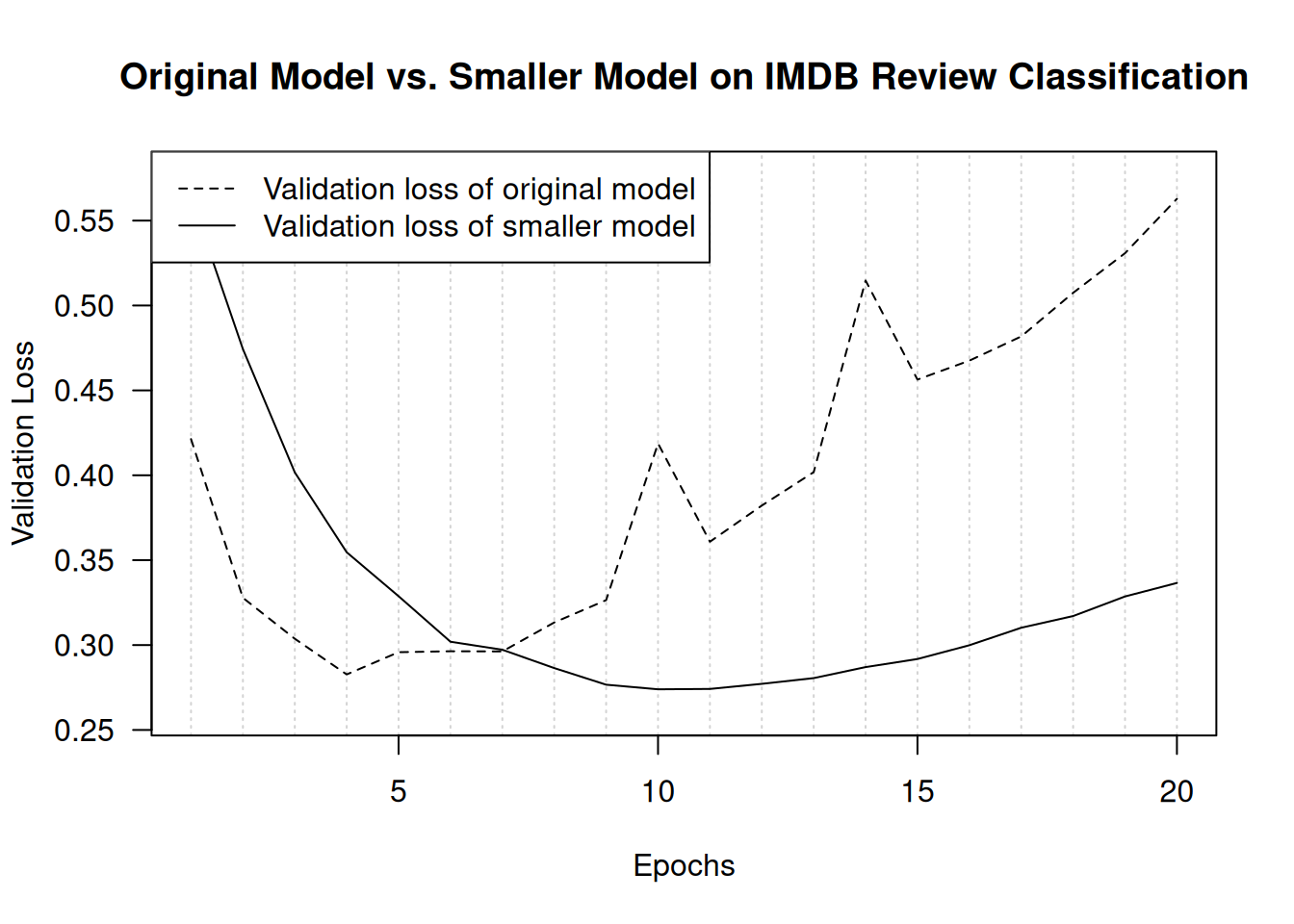
Now, let’s add to our benchmark a model that has much more capacity—far more than the problem warrants.
model <- keras_model_sequential() |>
  layer_dense(512, activation = "relu") |>
  layer_dense(512, activation = "relu") |>
  layer_dense(1, activation = "sigmoid")

model |> compile(
  optimizer = "rmsprop",
  loss = "binary_crossentropy",
  metrics = "accuracy"
)

history_larger_model <- model |> fit(
  train_data, train_labels,
  epochs = 20, batch_size = 512, validation_split = 0.4
)
Figure 5.19 shows how the bigger model fares compared to the reference model. It starts overfitting almost immediately, after just one epoch, and it overfits much more severely. Its validation loss is also noisier. It gets training loss near zero very quickly. The more capacity the model has, the more quickly it can model the training data (resulting in a low training loss), but the more susceptible it is to overfitting (resulting in a large difference between the training and validation loss).
plot(
  NULL,
  main = "Original Model vs. Much Larger Model on IMDB Review Classification",
  xlab = "Epochs", xlim = c(1, history_original$params$epochs),
  ylab = "Validation Loss",
  ylim = range(c(history_original$metrics$val_loss,
                 history_larger_model$metrics$val_loss)),
  panel.first = abline(v = 1:history_original$params$epochs,
                       lty = "dotted", col = "lightgrey")
)
lines(history_original    $metrics$val_loss, lty = 2)
lines(history_larger_model$metrics$val_loss, lty = 1)
legend("topleft", lty = 2:1,
       legend = c("Validation loss of original model",
                  "Validation loss of larger model"))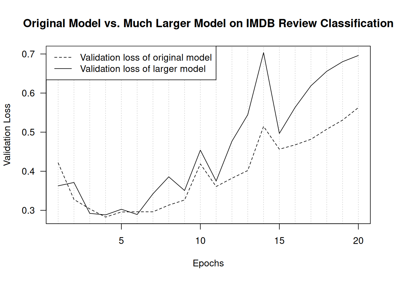
5.4.4.2 Adding weight regularization
You may be familiar with the principle of Occam’s razor: given two explanations for something, the explanation most likely to be correct is the simplest one—the one that makes fewer assumptions. This idea also applies to the models learned by neural networks: given some training data and a network architecture, multiple sets of weight values (multiple models) could explain the data. Simpler models are less likely to overfit than complex ones.
A simple model in this context is a model where the distribution of parameter values has less entropy (or a model with fewer parameters, as you saw in the previous section). Thus, a common way to mitigate overfitting is to put constraints on the complexity of a model by forcing its weights to take only small values, which makes the distribution of weight values more regular. This is called weight regularization, and it’s done by adding to the loss function of the model a cost associated with having large weights. This cost comes in two flavors:
- L1 regularization—The cost added is proportional to the absolute value of the weight coefficients (the L1 norm of the weights).
- L2 regularization—The cost added is proportional to the square of the value of the weight coefficients (the L2 norm of the weights). L2 regularization is also called weight decay in the context of neural networks. Don’t let the different name confuse you: weight decay is mathematically the same as L2 regularization.
In Keras, weight regularization is added by passing weight regularizer instances to layers as keyword arguments. Let’s add L2 weight regularization to the movie review classification model.
model <- keras_model_sequential() |>
  layer_dense(16, activation = "relu",
              kernel_regularizer = regularizer_l2(0.002)) |>
  layer_dense(16, activation = "relu",
              kernel_regularizer = regularizer_l2(0.002)) |>
  layer_dense(1, activation = "sigmoid")

model |> compile(
  optimizer = "rmsprop",
  loss = "binary_crossentropy",
  metrics = "accuracy"
)

history_l2_reg <- model |> fit(
  train_data, train_labels,
  epochs = 20, batch_size = 512, validation_split = 0.4
)
regularizer_l2(0.002) means every coefficient in the weight matrix of the layer will add 0.002 * weight_coefficient_value ^ 2 to the total loss of the model. Note that because this penalty is added only at training time, the loss for this model will be much higher at training than at test time.
Figure 5.20 shows the effect of the L2 regularization penalty. As you can see, the model with L2 regularization has become much more resistant to overfitting than the reference model, even though both models have the same number of parameters:
plot(NULL,
     main = "Effect of L2 Weight Regularization on Validation Loss",
     xlab = "Epochs", xlim = c(1, history_original$params$epochs),
     ylab = "Validation Loss",
     ylim = range(c(history_original$metrics$val_loss,
                    history_l2_reg  $metrics$val_loss)),
     panel.first = abline(v = 1:history_original$params$epochs,
                          lty = "dotted", col = "lightgrey"))
lines(history_original$metrics$val_loss, lty = 2)
lines(history_l2_reg  $metrics$val_loss, lty = 1)
legend("topleft", lty = 2:1,
       legend = c("Validation loss of original model",
                  "Validation loss of L2-regularized model"))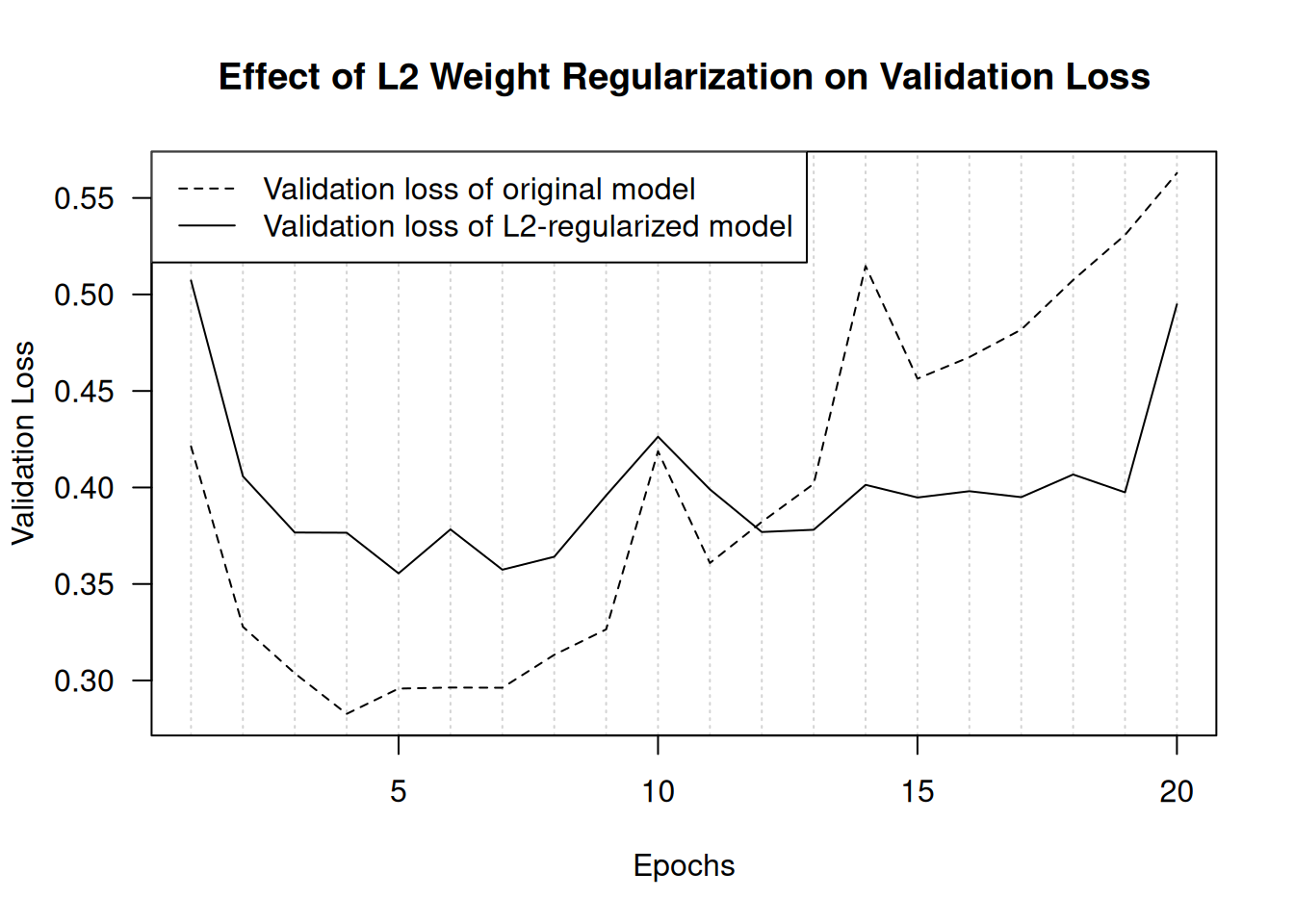
As an alternative to L2 regularization, we can use one of the following Keras weight regularizers.
- 1
- L1 regularization
- 2
- Simultaneous L1 and L2 regularization
Note that weight regularization is more typically used for smaller deep learning models. Large deep learning models tend to be so over-parameterized that imposing constraints on weight values does not have much effect on model capacity and generalization. In these cases, a different regularization technique is preferred: dropout.
5.4.4.3 Adding dropout
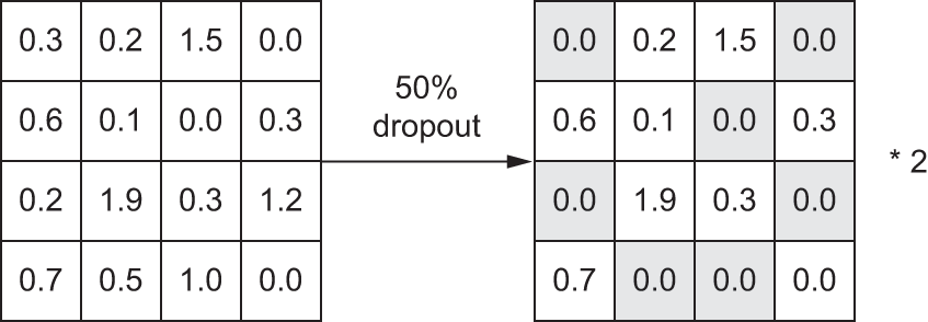
Dropout is one of the most effective and most commonly used regularization techniques for neural networks, developed by Geoff Hinton and his students at the University of Toronto. Dropout, applied to a layer, consists of randomly dropping out (setting to zero) a number of output features of the layer during training. Let’s say a given layer would normally return a vector c(0.2, 0.5, 1.3, 0.8, 1.1) for a given input sample during training. After applying dropout, this vector will have a few zero entries distributed at random: for example, c(0, 0.5, 1.3, 0, 1.1). The dropout rate is the fraction of the features that are zeroed out; it’s usually set between 0.2 and 0.5. At test time, no units are dropped out; instead, the layer’s output values are scaled down by a factor equal to 1 – dropout rate (the fraction of units kept) to balance the fact that more units are active than at training time.
Consider a matrix containing the output of a layer, layer_output, of shape (batch_size, features). At training time, we zero out at random a fraction of the values in the matrix:
1zero_out <- runif_array(dim(layer_output)) < .5
layer_output[zero_out] <- 0- 1
- At training time, drops out 50% of the units in the output
At test time, we scale down the output by the fraction of units kept (1 – dropout rate). Here, we scale by 0.5 (because we previously dropped half the units):
1layer_output <- layer_output * .5- 1
- At test time
Note that this process can be implemented by doing both operations at training time and leaving the output unchanged at test time, which is often the way it’s implemented in practice (see figure 5.21). In the figure, shaded entries indicate values that were set to 0 by dropout (not values that already happened to be 0):
- 1
- At training time
- 2
- Note that we’re scaling up rather than scaling down in this case.
This technique may seem strange and arbitrary. Why would this help reduce overfitting? Hinton says he was inspired by, among other things, a fraud-prevention mechanism used by banks:
I went to my bank. The tellers kept changing and I asked one of them why. He said he didn’t know but they got moved around a lot. I figured it must be because it would require cooperation between employees to successfully defraud the bank. This made me realize that randomly removing a different subset of neurons on each example would prevent conspiracies and thus reduce overfitting.
The core idea is that introducing noise in the output values of a layer can break up happenstance patterns that aren’t significant (what Hinton refers to as conspiracies), which the model will start memorizing if no noise is present.
In Keras, we can introduce dropout via layer_dropout(), which is applied to the output of the layer right before it. Let’s add two dropout layers to the IMDb model to see how well they do at reducing overfitting.
model <- keras_model_sequential() |>
  layer_dense(16, activation = "relu") |>
  layer_dropout(0.5) |>
  layer_dense(16, activation = "relu") |>
  layer_dropout(0.5) |>
  layer_dense(1, activation = "sigmoid")

model |> compile(
  optimizer = "rmsprop",
  loss = "binary_crossentropy",
  metrics = "accuracy"
)

history_dropout <- model |> fit(
  train_data, train_labels,
  epochs = 20, batch_size = 512,
  validation_split = 0.4
)
Figure 5.22 shows a plot of the results. This is a clear improvement over the reference model. It also seems to be working much better than L2 regularization because the lowest validation loss reached has improved:
plot(NULL,
     main = "Effect of Dropout on Validation Loss",
     xlab = "Epochs", xlim = c(1, history_original$params$epochs),
     ylab = "Validation Loss",
     ylim = range(c(history_original$metrics$val_loss,
                    history_dropout $metrics$val_loss)),
     panel.first = abline(v = 1:history_original$params$epochs,
                          lty = "dotted", col = "lightgrey"))
lines(history_original$metrics$val_loss, lty = 2)
lines(history_dropout $metrics$val_loss, lty = 1)
legend("topleft", lty = 2:1,
       legend = c("Validation loss of original model",
                  "Validation loss of dropout-regularized model"))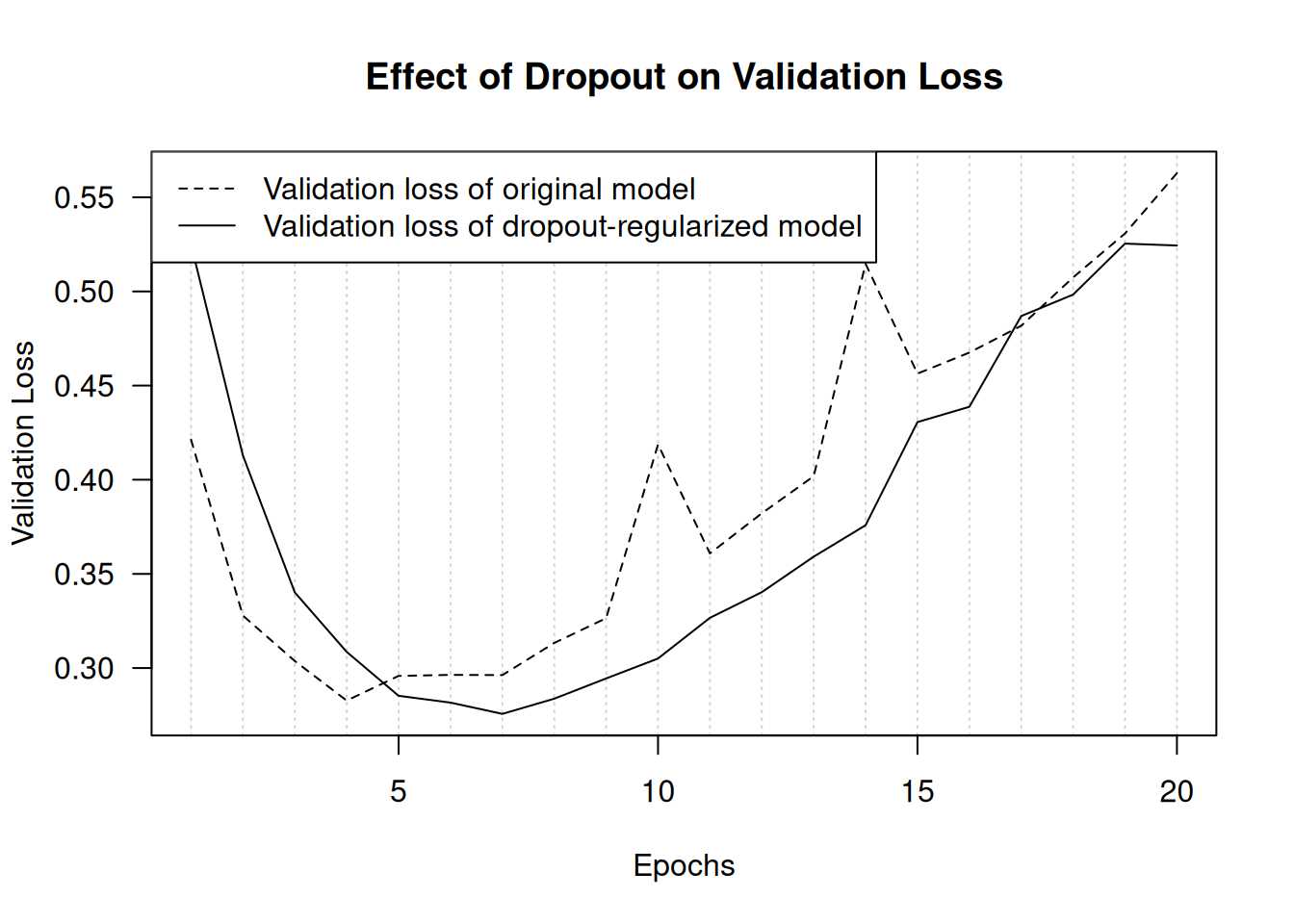
To recap, these are the most common ways to maximize generalization and prevent overfitting in neural networks:
- Getting more training data, or better training data
- Developing better features
- Reducing the capacity of the model
- Adding weight regularization (for smaller models)
- Adding dropout
5.5 Summary
- The purpose of a machine learning model is to generalize: to perform accurately on never-before-seen inputs. It’s harder than it seems.
- A deep neural network achieves generalization by learning a parametric model that can successfully interpolate between training samples. Such a model can be said to have learned the latent manifold of the training data. This is why deep learning models can only make sense of inputs that are very close to what they’ve seen during training.
- The fundamental problem in machine learning is the tension between optimization and generalization: to attain generalization, you must first achieve a good fit to the training data, but improving your model’s fit to the training data will inevitably start hurting generalization after a while. Every single deep learning best practice deals with managing this tension.
- The ability of deep learning models to generalize comes from the fact that they manage to learn to approximate the latent manifold of their data and can thus make sense of new inputs via interpolation.
- It’s essential to be able to accurately evaluate the generalization power of your model while you’re developing it. You have at your disposal an array of evaluation methods, from simple hold-out validation to K-fold cross-validation and iterated K-fold cross-validation with shuffling. Remember to always keep a completely separate test set for final model evaluation, because information leaks from your validation data to your model may have occurred.
- When you start working on a model, your goal is first to achieve a model that has some generalization power and that can overfit. Best practices to do this include tuning your learning rate and batch size, using better architecture priors, increasing model capacity, or simply training longer.
- As your model starts overfitting, your goal switches to improving generalization through model regularization. You can reduce your model’s capacity, add dropout or weight regularization, and use early stopping. And naturally, a larger or better dataset is always the number one way to help a model generalize.