

library(tensorflow, exclude = c("shape", "set_random_seed"))
library(tfdatasets, exclude = "shape")
library(dplyr, warn.conflicts = FALSE)
library(keras3)

url <- paste0(
  "https://s3.amazonaws.com/keras-datasets/",
  "jena_climate_2009_2016.csv.zip"
)
get_file(origin = url) |>
zip::unzip("jena_climate_2009_2016.csv")13 Timeseries forecasting
This chapter covers
- An overview of machine learning for timeseries
- Understanding recurrent neural networks (RNNs)
- Applying RNNs to a temperature forecasting example
This chapter tackles timeseries, where temporal order is everything. We’ll focus on the most common and valuable timeseries task: forecasting. Using the recent past to predict the near future is a powerful capability, whether we’re trying to anticipate energy demand, manage inventory, or simply forecast the weather.
13.1 Different kinds of timeseries tasks
A timeseries can be any data obtained via measurements at regular intervals, like the daily price of a stock, the hourly electricity consumption of a city, or the weekly sales of a store. Timeseries are everywhere, whether we’re looking at natural phenomena (like seismic activity, the evolution of fish populations in a river, or the weather at a location) or human activity patterns (such as visitors to a website, a country’s GDP, or credit card transactions). Unlike the types of data you’ve encountered so far, working with timeseries involves understanding the dynamics of a system: its periodic cycles, how it trends over time, its regular regime, and its sudden spikes.
By far, the most common timeseries-related task is forecasting—predicting what happens next in the series: for example, forecasting electricity consumption a few hours in advance so we can anticipate demand, forecasting revenue a few months in advance so we can plan our budget, or forecasting the weather a few days in advance so we can plan our schedule. Forecasting is what this chapter focuses on. But there’s actually a wide range of other things we can do with timeseries, such as these:
- Anomaly detection—Detect anything unusual happening within a continuous data stream. Unusual activity on our corporate network? Might be an attacker. Unusual readings on a manufacturing line? Time for a human to go take a look. Anomaly detection is typically done via unsupervised learning, because we often don’t know what kind of anomaly we’re looking for, and thus we can’t train on specific anomaly examples.
- Classification—Assign one or more categorical labels to a timeseries. For instance, given the timeseries of activity of a visitor on a website, classify whether the visitor is a bot or a human.
- Event detection—Identify the occurrence of a specific, expected event within a continuous data stream. A particularly useful application is hotword detection, where a model monitors an audio stream and detects utterances like “OK, Google” and “Hey, Alexa.”
In this chapter, you’ll learn about recurrent neural networks (RNNs) and how to apply them to timeseries forecasting. Then, in the next chapter, you’ll learn all about anomaly detection.
13.2 A temperature forecasting example
Throughout this chapter, all of our code examples will target a single problem: predicting the temperature 24 hours in the future, given a timeseries of hourly measurements of quantities such as atmospheric pressure and humidity, recorded over the recent past by a set of sensors on the roof of a building. As you will see, it’s a fairly challenging problem!
We’ll use this temperature forecasting task to highlight what makes timeseries data fundamentally different from the kinds of datasets you’ve encountered so far, to show that densely connected networks and convolutional networks aren’t well-equipped to deal with it, and to demonstrate a new kind of machine learning technique that really shines on this type of problem: RNNs. We’ll work with a weather timeseries dataset recorded at the Weather Station at the Max Planck Institute for Biogeochemistry in Jena, Germany.1 In this dataset, 14 different quantities (such as temperature, pressure, humidity, wind direction, and so on) were recorded every 10 minutes over several years. The original data goes back to 2003, but the subset of the data we’ll download is limited to 2009–2016.
Let’s start by downloading and uncompressing the data:
Now, let’s look at the data.
writeLines(readLines("jena_climate_2009_2016.csv", 3))"Date Time","p (mbar)","T (degC)","Tpot (K)","Tdew (degC)","rh (%)","VPmax (mbar)","VPact (mbar)","VPdef (mbar)","sh (g/kg)","H2OC (mmol/mol)","rho (g/m**3)","wv (m/s)","max. wv (m/s)","wd (deg)"
01.01.2009 00:10:00,996.52,-8.02,265.40,-8.90,93.30,3.33,3.11,0.22,1.94,3.12,1307.75,1.03,1.75,152.30
01.01.2009 00:20:00,996.57,-8.41,265.01,-9.28,93.40,3.23,3.02,0.21,1.89,3.03,1309.80,0.72,1.50,136.10withr::with_package("readr", {
full_df <- read_csv(
"jena_climate_2009_2016.csv",
locale = locale(tz = "Etc/GMT+1"),
col_types = cols(
`Date Time` = col_datetime("%d.%m.%Y %H:%M:%S"),
.default = col_double()
)
)
})This outputs a data.frame with 420,451 rows and 15 columns. Each row is a time step: a record of a date and 14 weather-related values. We won’t be training on the Date Time column, but for completeness, we parse it as a POSIXct with the correct time zone. We pass tz = "Etc/GMT+1" instead of tz = "Europe/Berlin" because the timestamps in the dataset do not adjust for Central European Summer Time (also known as Daylight Saving Time) and are always in Central European Time.
tibble::glimpse(full_df)Rows: 420,451
Columns: 15
$ `Date Time` <dttm> 2009-01-01 00:10:00, 2009-01-01 00:20:00, 2009-…
$ `p (mbar)` <dbl> 996.52, 996.57, 996.53, 996.51, 996.51, 996.50, …
$ `T (degC)` <dbl> -8.02, -8.41, -8.51, -8.31, -8.27, -8.05, -7.62,…
$ `Tpot (K)` <dbl> 265.40, 265.01, 264.91, 265.12, 265.15, 265.38, …
$ `Tdew (degC)` <dbl> -8.90, -9.28, -9.31, -9.07, -9.04, -8.78, -8.30,…
$ `rh (%)` <dbl> 93.3, 93.4, 93.9, 94.2, 94.1, 94.4, 94.8, 94.4, …
$ `VPmax (mbar)` <dbl> 3.33, 3.23, 3.21, 3.26, 3.27, 3.33, 3.44, 3.44, …
$ `VPact (mbar)` <dbl> 3.11, 3.02, 3.01, 3.07, 3.08, 3.14, 3.26, 3.25, …
$ `VPdef (mbar)` <dbl> 0.22, 0.21, 0.20, 0.19, 0.19, 0.19, 0.18, 0.19, …
$ `sh (g/kg)` <dbl> 1.94, 1.89, 1.88, 1.92, 1.92, 1.96, 2.04, 2.03, …
$ `H2OC (mmol/mol)` <dbl> 3.12, 3.03, 3.02, 3.08, 3.09, 3.15, 3.27, 3.26, …
$ `rho (g/m**3)` <dbl> 1307.75, 1309.80, 1310.24, 1309.19, 1309.00, 130…
$ `wv (m/s)` <dbl> 1.03, 0.72, 0.19, 0.34, 0.32, 0.21, 0.18, 0.19, …
$ `max. wv (m/s)` <dbl> 1.75, 1.50, 0.63, 0.50, 0.63, 0.63, 0.63, 0.50, …
$ `wd (deg)` <dbl> 152.3, 136.1, 171.6, 198.0, 214.3, 192.7, 166.5,…
Let’s plot the temperature (in degrees Celsius) over time (see Figure 13.1). On this plot, you can clearly see the yearly periodicity of temperature; the data spans eight years.
plot(`T (degC)` ~ `Date Time`, data = full_df, pch = 20, cex = .3)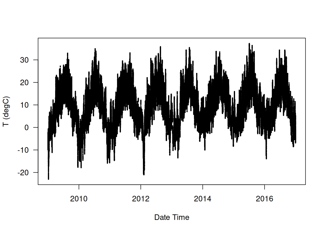
Now let’s look at a narrower plot of the first 10 days of temperature data (figure 13.2). Because the data is recorded every 10 minutes, we get 24 × 6 = 144 data points per day.
plot(`T (degC)` ~ `Date Time`, data = full_df[1:1440, ])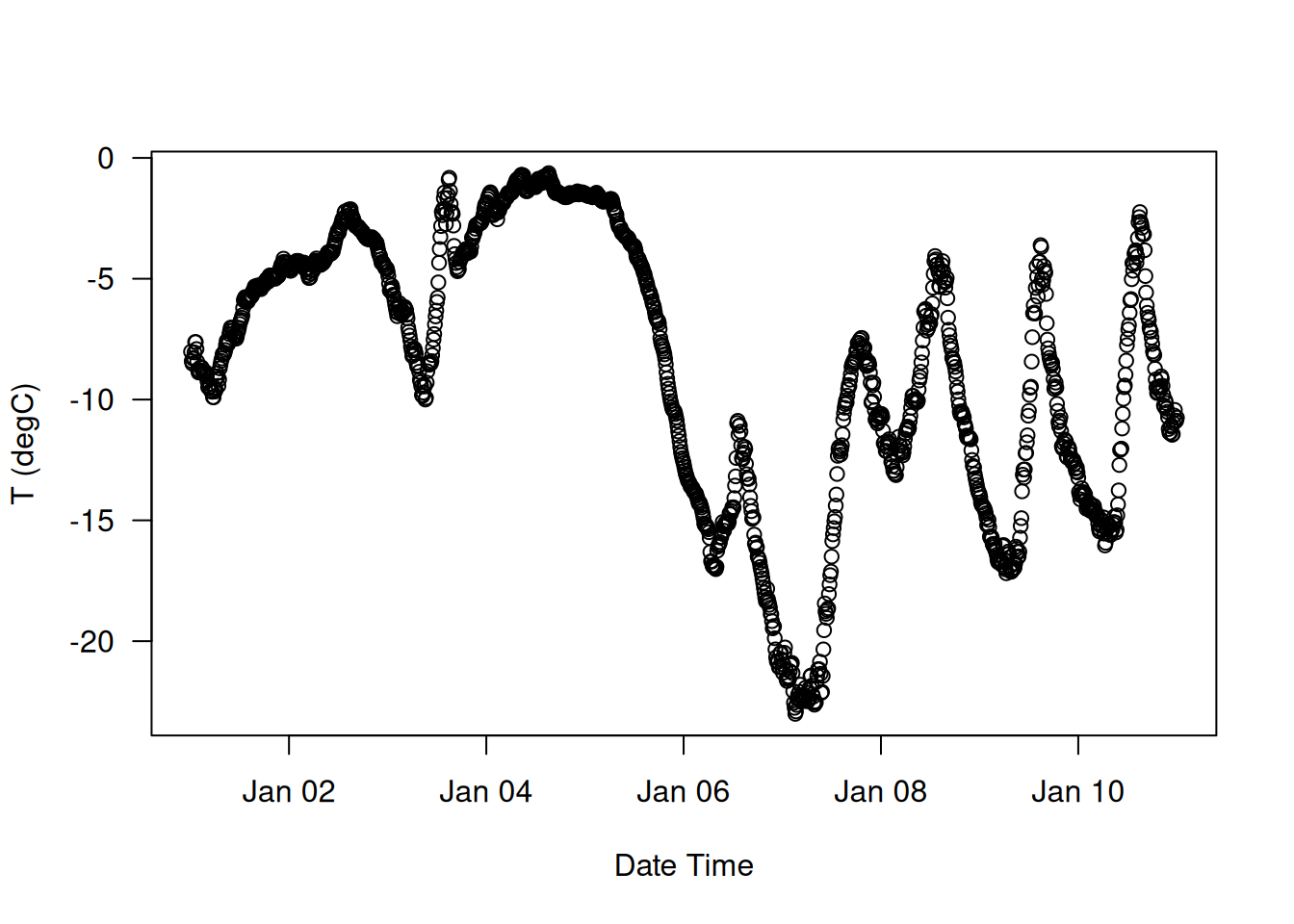
On this plot, you can see daily periodicity, which is especially evident for the last four days. Also note that this 10-day period must come from a fairly cold winter month.
NoteAlways look for periodicity in your data
Periodicity over multiple timescales is an important and very common property of timeseries data. Whether you’re looking at the weather, mall parking occupancy, traffic to a website, sales of a grocery store, or steps logged in a fitness tracker, you’ll see daily cycles and yearly cycles (human-generated data also tends to feature weekly cycles). When exploring your data, be sure to look for these patterns.
With our dataset, if we were trying to predict the average temperature for the next month given a few months of past data, the problem would be easy, due to the reliable year-scale periodicity of the data. But looking at the data over a scale of days, the temperature looks a lot more chaotic. Is this timeseries predictable at a daily scale? Let’s find out.
In all our experiments, we’ll use the first 50% of the data for training, the next 25% for validation, and the last 25% for testing. When working with timeseries data, it’s important to use validation and test data that is more recent than the training data because we’re trying to predict the future given the past, not the reverse, and our validation/test splits should reflect this temporal ordering. Some problems happen to be considerably simpler if we reverse the time axis!
num_train_samples <- round(nrow(full_df) * .5)
num_val_samples <- round(nrow(full_df) * 0.25)
num_test_samples <- nrow(full_df) - num_train_samples - num_val_samples

train_df <- full_df[seq(num_train_samples), ]

val_df <- full_df[seq(from = nrow(train_df) + 1,
                      length.out = num_val_samples), ]

test_df <- full_df[seq(to = nrow(full_df),
                       length.out = num_test_samples), ]

cat("num_train_samples:", nrow(train_df), "\n")
cat("num_val_samples:", nrow(val_df), "\n")
cat("num_test_samples:", nrow(test_df), "\n")
num_train_samples: 210226
num_val_samples: 105113
num_test_samples: 105112 13.2.1 Preparing the data
The exact formulation of the problem will be as follows: given data covering the previous five days and sampled once per hour, can we predict the temperature in 24 hours?
First, let’s preprocess the data into a format a neural network can ingest. This is easy: the data is already numerical, so we don’t need to do any vectorization. But each timeseries in the data is on a different scale (for example, atmospheric pressure, measured in mbar, is around 1,000, whereas H2OC, measured in millimoles per mole, is around 3). We’ll normalize each timeseries independently so that they all take small values on a similar scale. We’re going to use the first 210,226 timesteps as training data, so we’ll compute the mean and standard deviation on only this fraction of the data.
input_data_colnames <- names(full_df) |> setdiff(c("Date Time"))
normalization_values <- train_df[input_data_colnames] |>
  lapply(\(col) list(mean = mean(col), sd = sd(col)))

str(normalization_values)
List of 14
$ p (mbar) :List of 2
..$ mean: num 989
..$ sd : num 8.51
$ T (degC) :List of 2
..$ mean: num 8.83
..$ sd : num 8.77
$ Tpot (K) :List of 2
..$ mean: num 283
..$ sd : num 8.87
$ Tdew (degC) :List of 2
..$ mean: num 4.31
..$ sd : num 7.08
$ rh (%) :List of 2
..$ mean: num 75.9
..$ sd : num 16.6
[list output truncated]normalize_input_data <- function(df) {
purrr::map2(df, normalization_values[names(df)], \(col, nv) {
(col - nv$mean) / nv$sd
}) |> as_tibble()
}Next, let’s create a Dataset object that yields batches of data from the past 5 days along with a target temperature 24 hours in the future. Because the samples in the dataset are highly redundant (sample N and sample N + 1 will have most of their timesteps in common), it would be wasteful to explicitly allocate memory for every sample. Instead, we’ll generate the samples on the fly while only keeping in memory the original input features and temperature targets, and nothing more.
We could easily write a tfdataset or R generator (with coro::generator() or py_iterator()) to do this. But Keras has a built-in dataset utility that does what we need (timeseries_dataset_from_array()), so we can save ourselves some work by using it. You can generally use it for any kind of timeseries forecasting task.
NoteUnderstanding
timeseries_dataset_from_array()
To understand what timeseries_dataset_from_array() does, let’s take a look at a simple example. The general idea is that we provide an array of timeseries data (the data argument), and timeseries_dataset_from_array gives us windows extracted from the original timeseries (we’ll call them sequences).
Let’s say we’re using data = [1 2 3 4 5 6] and sequence_length=3. Then timeseries_dataset_from_array will generate the following samples: [1 2 3], [2 3 4], [3 4 5], [4 5 6].
We can also pass a target array to timeseries_dataset_from_array(). The first entry of the targets array should match the desired target for the first sequence that will be generated from the data array. So if we’re doing timeseries forecasting, we use as targets the same array as for data, offset by some amount.
For instance, with data = [1 2 3 4 5 6 7...] and sequence_length=3, we can create a dataset to predict the next step in the series by passing targets = [4 5 6 7...]. Let’s try it:
int_sequence <- seq(10)
dummy_dataset <- timeseries_dataset_from_array(
  data = head(int_sequence, -3),
  targets = tail(int_sequence, -3),
  sequence_length = 3,
  batch_size = 2
)

dummy_dataset_iterator <- as_array_iterator(dummy_dataset)

repeat {
  batch <- iter_next(dummy_dataset_iterator)
  if (is.null(batch)) break
  .[inputs, targets] <- batch
  for (r in 1:nrow(inputs))
    cat(sprintf("input: [ %s ]  target: %s\n",
                paste(inputs[r, ], collapse = " "), targets[r]))
  cat(strrep("-", 27), "\n")
}
input: [ 1 2 3 ] target: 4
input: [ 2 3 4 ] target: 5
---------------------------
input: [ 3 4 5 ] target: 6
input: [ 4 5 6 ] target: 7
---------------------------
input: [ 5 6 7 ] target: 8
--------------------------- Here’s what this short snippet is doing, step by step: 1. It generates an array of sorted integers from 1 to 10. 2. The sequences we generate will be sampled from [1 2 3 4 5 6 7]. 3. The target for the sequence that starts at data[N] will be data[N + 3]. 4. The sequences will be three steps long. 5. The sequences will be batched in batches of size 2.
We’ll use timeseries_dataset_from_array() to instantiate three datasets: one for training, one for validation, and one for testing.
We’ll use the following parameter values:
sampling_rate = 6—Observations will be sampled at one data point per hour: we will only keep one data point out of six.sequence_length = 120—Observations will go back 5 days (120 hours).delay = sampling_rate * (sequence_length + 24 - 1)—The target for a sequence will be the temperature 24 hours after the end of the sequence.start_index = 0andend_index = num_train_samples—For the training dataset, we’ll use only the first 50% of the data.start_index = num_train_samplesandend_index = num_train_samples + num_val_samples—For the validation dataset, we’ll use only the next 25% of the data.start_index = num_train_samples + num_val_samples—For the test dataset, we’ll use the remaining samples.
sampling_rate <- 6
sequence_length <- 120
delay <- sampling_rate * (sequence_length + 24 - 1)
batch_size <- 256

df_to_inputs_and_targets <- function(df) {
  inputs <- df[input_data_colnames] |>
    normalize_input_data() |>
    as.matrix()

  targets <- as.array(df$`T (degC)`)

  list(
    head(inputs, -delay),
    tail(targets, -delay)
  )
}

make_dataset <- function(df) {
  .[inputs, targets] <- df_to_inputs_and_targets(df)

  timeseries_dataset_from_array(
    inputs, targets,
    sampling_rate = sampling_rate,
    sequence_length = sequence_length,
    shuffle = TRUE,
    batch_size = batch_size
  )
}

train_dataset <- make_dataset(train_df)
val_dataset <- make_dataset(val_df)
test_dataset <- make_dataset(test_df)
Each dataset yields a tuple (samples, targets), where samples is a batch of 256 samples, each containing 120 consecutive hours of input data, and targets is the corresponding array of 256 target temperatures. Note that the samples are randomly shuffled, so two consecutive sequences in a batch (like samples[1] and samples[2]) aren’t necessarily temporally close.
.[samples, targets] <- iter_next(as_iterator(train_dataset))
cat("samples shape: ", format(samples$shape), "\n",
    "targets shape: ", format(targets$shape), "\n", sep = "")
samples shape: (256, 120, 14)
targets shape: (256)13.2.2 A common-sense, non-machine-learning baseline
Before we start using black-box deep learning models to solve the temperature prediction problem, let’s try a simple, common-sense approach. It will serve as a sanity check, and it will establish a baseline that we’ll have to beat to demonstrate the usefulness of more advanced machine learning models. Such common-sense baselines can be useful when we’re approaching a new problem for which there is no known solution (yet). A classic example is unbalanced classification tasks, where some classes are much more common than others. If a dataset contains 90% instances of class A and 10% instances of class B, then a common-sense approach to the classification task is to always predict “A” when presented with a new sample. Such a classifier is 90% accurate overall, and any learning-based approach should therefore beat this 90% score to demonstrate usefulness. Sometimes, such elementary baselines can prove surprisingly hard to beat.
In this case, the temperature timeseries can safely be assumed to be continuous (the temperatures tomorrow are likely to be close to the temperatures today) as well as periodic, with a daily period. Thus, a common-sense approach is to always predict that the temperature 24 hours from now will be equal to the temperature right now. Let’s evaluate this approach, using the mean absolute error (MAE) metric, defined as follows:
mean(abs(preds - targets))Rather than evaluating all the data eagerly in R using for, as_array_iterator(), and iter_next(), we can just as easily do it using tfdataset functions. First we call dataset_unbatch() so that each dataset element becomes a single case of (samples, target). Next we use dataset_map() to calculate the absolute error for each pair of (samples, target) and then dataset_reduce() to accumulate the total error and total samples seen.
Recall that functions passed to dataset_map() and dataset_reduce() will be called with symbolic tensors. Slicing a tensor like samples@r[-1, ] selects the last slice along that axis, as if we had written samples[nrow(samples), ].
evaluate_naive_method <- function(dataset) {

  .[temp_sd = sd, temp_mean = mean] <- normalization_values$`T (degC)`
  unnormalize_temperature <- function(x) {
    (x * temp_sd) + temp_mean
  }

  temp_col_idx <- match("T (degC)", input_data_colnames)

  reduction <- dataset |>
    dataset_unbatch() |>
    dataset_map(function(samples, target) {
1      last_temp_in_input <- samples@r[-1, temp_col_idx]
2      pred <- unnormalize_temperature(last_temp_in_input)
      abs(pred - target)
    }) |>
    dataset_reduce(
      initial_state = list(total_samples_seen = 0L,
                           total_abs_error = 0),
      reduce_func = function(state, element) {
        `add<-` <- `+`
        add(state$total_samples_seen) <- 1L
        add(state$total_abs_error) <- element
        state
      }
    ) |>
3    lapply(as.numeric)

4  mae <- with(reduction, total_abs_error / total_samples_seen)
  mae
}

sprintf("Validation MAE: %.2f", evaluate_naive_method(val_dataset))
sprintf("Test MAE: %.2f", evaluate_naive_method(test_dataset))- 1
- Slice out the last temperature measurement in the input sequence.
- 2
- Recall that we normalized our features, so to retrieve a temperature in Celsius, we need to unnormalize it by multiplying by the standard deviation and adding back the mean.
- 3
- Convert tensors to R numerics.
- 4
-
reductionis a named list of two R scalar numbers.
[1] "Validation MAE: 2.43"
[1] "Test MAE: 2.62"
This common-sense baseline achieves a validation MAE of 2.43 degrees Celsius and a test MAE of 2.62 degrees Celsius. So if we always assume that the temperature 24 hours in the future will be the same as it is now, we will be off by two and a half degrees on average. That’s not too bad, but we probably won’t launch a weather forecasting service based on this heuristic. Now, the game is to use your knowledge of deep learning to do better.
13.2.3 Let’s try a basic machine learning model
In the same way that it’s useful to establish a common-sense baseline before trying machine learning approaches, it’s useful to try simple, cheap machine learning models (such as small, densely connected networks) before looking into complicated and computationally expensive models such as RNNs. This is the best way to make sure any further complexity you throw at the problem is legitimate and delivers real benefits.
The next listing shows a fully connected model that starts by flattening the data and then runs it through two Dense layers. Note the lack of activation function on the last Dense layer, which is typical for a regression problem. We use mean squared error (MSE) as the loss, rather than MAE, because, unlike MAE, it’s smooth around zero, a useful property for gradient descent. We will monitor MAE by adding it as a metric in compile().
ncol_input_data <- length(input_data_colnames)

inputs <- keras_input(shape = c(sequence_length, ncol_input_data))
outputs <- inputs |>
1  layer_reshape(-1) |>
  layer_dense(16, activation="relu") |>
  layer_dense(1)

model <- keras_model(inputs, outputs)

callbacks = list(
2  callback_model_checkpoint("jena_dense.keras", save_best_only = TRUE)
)

model |> compile(
  optimizer = "adam",
  loss = "mse",
  metrics = "mae"
)

history <- model |> fit(
  train_dataset,
  epochs = 10,
  validation_data = val_dataset,
  callbacks = callbacks
)

3model <- load_model("jena_dense.keras")
sprintf("Test MAE: %.2f", evaluate(model, test_dataset)["mae"])- 1
- Flattens features
- 2
- Uses a callback to save the best-performing model
- 3
- Reloads the best model and evaluates it on the test data
[1] "Test MAE: 2.67"Let’s display the loss curves for training and validation (see figure 13.3).
plot(history, metrics = "mae")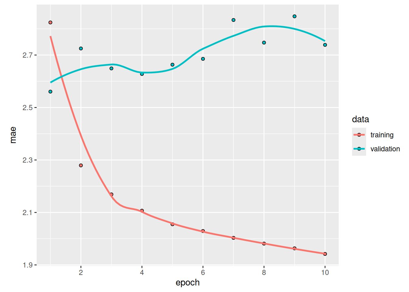
Some of the validation losses are close to the no-learning baseline, but not reliably. This goes to show the merit of having this baseline in the first place: it turns out to be not easy to outperform. Our common sense contains a lot of valuable information to which a machine learning model doesn’t have access.
You may wonder: if a simple, well-performing model exists to go from the data to the targets (the common-sense baseline), why doesn’t the model we’re training find it and improve on it? Well, the space of models in which we’re searching for a solution—that is, our hypothesis space—is the space of all possible two-layer networks with the configuration we defined. The common-sense heuristic is just one model among millions that can be represented in this space. It’s like looking for a needle in a haystack. Just because a good solution technically exists in our hypothesis space doesn’t mean we’ll be able to find it via gradient descent.
That’s a pretty significant limitation of machine learning in general: unless the learning algorithm is hardcoded to look for a specific kind of simple model, it can sometimes fail to find a simple solution to a simple problem. That’s why using good feature engineering and relevant architecture priors is essential: we need to precisely tell our model what it should be looking for.
13.2.4 Let’s try a 1D convolutional model
Speaking of using the right architecture priors, because our input sequences feature daily cycles, perhaps a convolutional model could work. A temporal convnet could reuse the same representations across different days, much like a spatial convnet can reuse the same representations across different locations in an image.
You already know about the Conv2D and SeparableConv2D layers, which see their inputs through small windows that swipe across 2D grids. There are also 1D and even 3D versions of these layers: Conv1D, SeparableConv1D, and Conv3D. (There isn’t a SeparableConv3D layer—not for any theoretical reason, but simply because we haven’t implemented it.) The Conv1D layer relies on 1D windows that slide across input sequences, and the Conv3D layer relies on cubic windows that slide across input volumes.
We can thus build 1D convnets, which are strictly analogous to 2D convnets. They’re a great fit for any sequence data that follows the translation invariance assumption (meaning that if we slide a window over the sequence, the content of the window should follow the same properties independently of the location of the window).
Let’s try one on our temperature forecasting problem. We’ll pick an initial window length of 24, so that we look at 24 hours of data at a time (one cycle). As we downsample the sequences (via MaxPooling1D layers), we’ll reduce the window size accordingly:
inputs <- keras_input(shape = c(sequence_length, ncol_input_data))
outputs <- inputs |>
  layer_conv_1d(8, 24, activation = "relu") |>
  layer_max_pooling_1d(2) |>
  layer_conv_1d(8, 12, activation = "relu") |>
  layer_max_pooling_1d(2) |>
  layer_conv_1d(8, 6, activation = "relu") |>
  layer_global_average_pooling_1d() |>
  layer_dense(1)
model <- keras_model(inputs, outputs)

callbacks <- list(
  callback_model_checkpoint("jena_conv.keras", save_best_only = TRUE)
)

model |> compile(
  optimizer = "adam",
  loss = "mse",
  metrics = "mae"
)
history <- model |> fit(
train_dataset,
epochs = 10,
validation_data = val_dataset,
callbacks = callbacks
)model <- load_model("jena_conv.keras")
sprintf("Test MAE: %.2f", evaluate(model, test_dataset)[["mae"]])[1] "Test MAE: 3.06"plot(history, metrics = "mae")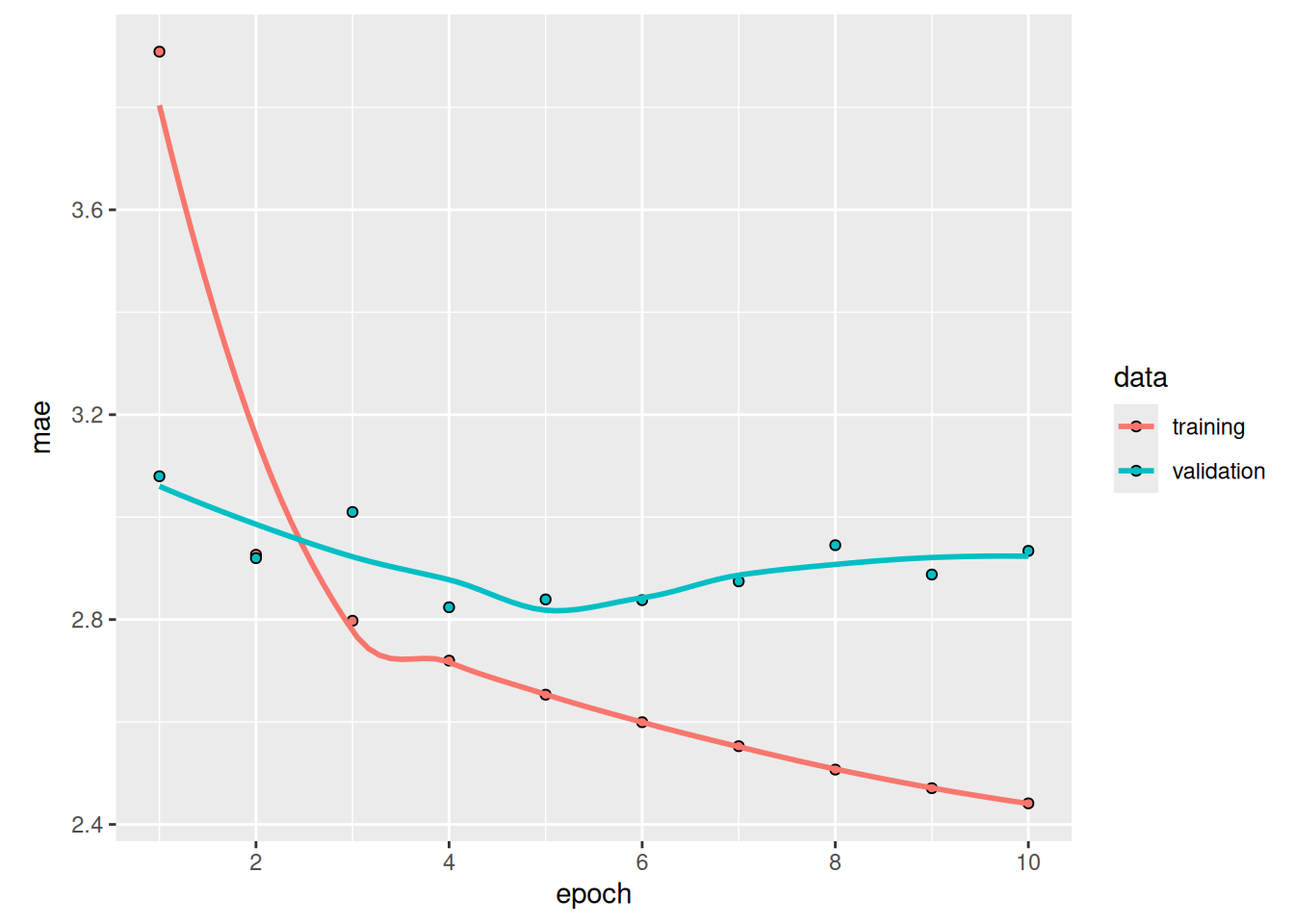
As it turns out, this model performs even worse than the densely connected one: it achieves a validation MAE of only about 2.9 degrees, far from the common-sense baseline (figure 13.4). What went wrong here? Two things:
- Weather data doesn’t respect the translation invariance assumption. Although the data does feature daily cycles, data from a morning follows different properties than data from an evening or from the middle of the night. Weather data is only translation invariant for a very specific timescale.
- Order in our data matters—a lot. The recent past is far more informative for predicting the next day’s temperature than data from five days ago. A 1D convnet can’t use this fact. In particular, our max pooling and global average pooling layers are largely destroying order information.
13.3 RNNs
Neither the fully connected approach nor the convolutional approach did well, but that doesn’t mean machine learning isn’t applicable to this problem. The densely connected approach first flattened the timeseries, which removed the notion of time from the input data. The convolutional approach treated every segment of the data the same way, even applying pooling, which destroyed order information. Let’s instead look at the data as what it is: a sequence, where causality and order matter.
There’s a family of neural network architectures that were designed specifically for this use case: RNNs. Among them, the long short-term memory (LSTM) layer in particular is very popular. We’ll see in a minute how these models work—but let’s start by giving the LSTM layer a try (see figure 13.5).
inputs <- keras_input(shape = c(sequence_length, ncol_input_data))
outputs <- inputs |>
  layer_lstm(16) |>
  layer_dense(1)
model <- keras_model(inputs, outputs)

callbacks <- list(
  callback_model_checkpoint("jena_lstm.keras", save_best_only = TRUE)
)

compile(model, optimizer = "adam", loss = "mse", metrics = "mae")
history <- model |> fit(
train_dataset,
epochs = 10,
validation_data = val_dataset,
callbacks = callbacks
)![Training and validation MAE on the Jena temperature-forecasting task with an LSTM-based model (note that we omit epoch 1 on this graph, because the high training MAE [7.75] at epoch 1 would distort the scale)](chapter13_timeseries-forecasting_files/figure-html/plot_lstm_forecast_mae-1.png)
model <- load_model("jena_lstm.keras")
sprintf("Test MAE: %.2f", evaluate(model, test_dataset)[["mae"]])
[1] "Test MAE: 2.49"Much better! We achieve a validation MAE as low as 2.39 degrees and a test MAE of 2.55 degrees. The LSTM-based model can finally beat the common-sense baseline (albeit only by a bit, for now), demonstrating the value of machine learning on this task.
But why did the LSTM model perform markedly better than the densely connected one or the convnet? And how can we further refine the model? To answer this, let’s take a closer look at RNNs.
13.3.1 Understanding RNNs
A major characteristic of all neural networks you’ve seen so far, such as densely connected networks and convnets, is that they have no memory. Each input shown to them is processed independently, with no state kept in between inputs. With such networks, to process a sequence or a temporal series of data points, we have to show the entire sequence to the network at once: turn it into a single data point. For instance, this is what we did in the densely connected network example: we flattened our five days of data into a single large vector and processed it in one go. Such networks are called feedforward networks.
In contrast, as you’re reading the present sentence, you’re processing it word by word—or rather, eye saccade by eye saccade—while keeping memories of what came before; this gives you a fluid representation of the meaning conveyed by this sentence. Biological intelligence processes information incrementally while maintaining an internal model of what it’s processing, built from past information and constantly updated as new information comes in.
An RNN adopts the same principle, albeit in an extremely simplified version: it processes sequences by iterating through the sequence elements and maintaining a state containing information relative to what it has seen so far. In effect, an RNN is a type of neural network that has an internal loop (see figure 13.6).
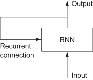
The state of the RNN is reset between processing two different, independent sequences (such as two samples in a batch), so we still consider one sequence to be a single data point: a single input to the network. What changes is that this data point is no longer processed in a single step; rather, the network internally loops over sequence elements.
To make these notions of loop and state clear, let’s implement the forward pass of a toy RNN. This RNN takes as input a sequence of vectors, which we’ll encode as a rank-2 tensor of size (timesteps, input_features). It loops over timesteps, and at each timestep, it considers its current state at t and the input at t (of shape (input_features)) and combines them to obtain the output at t. We’ll then set the state for the next step to be this previous output. For the first timestep, the previous output isn’t defined; hence, there is no current state. So, we’ll initialize the state as an all-zero vector called the initial state of the network. The following listing shows the RNN in pseudocode.
- 1
-
The state at
t - 2
- Iterates over sequence elements
- 3
- The previous output becomes the state for the next iteration.
We can even flesh out the function f: the transformation of the input and state into an output will be parameterized by two matrices, W and U, and a bias vector. It’s similar to the transformation operated by a densely connected layer in a feedforward network.
state_t <- 0
for (input_t in input_sequence) {
  output_t <- activation(dot(W, input_t) + dot(U, state_t) + b)
  state_t <- output_t
}
To make these notions absolutely unambiguous, let’s write a naive R implementation of the forward pass of the simple RNN.
runif_array <- function(dim) array(runif(prod(dim)), dim)

1timesteps <- 100
2input_features <- 32
3output_features <- 64

4inputs <- runif_array(c(timesteps, input_features))
5state_t <- array(0, dim = output_features)
6W <- runif_array(c(output_features, input_features))
U <- runif_array(c(output_features, output_features))
b <- runif_array(c(output_features, 1))
outputs <- array(0, dim = c(timesteps, output_features))

for(ts in 1:timesteps) {
7  input_t <- inputs[ts, ]
8  output_t <- tanh( (W %*% input_t) + (U %*% state_t) + b )
9  outputs[ts, ] <- state_t <- output_t
}

10final_output_sequence <- outputs- 1
- Number of timesteps in the input sequence
- 2
- Dimensionality of the input feature space
- 3
- Dimensionality of the output feature space
- 4
- Input data: random noise for the sake of the example
- 5
- Initial state: an all-zero vector
- 6
- Creates random weight matrices
- 7
-
input_tis a vector of shape(input_features). - 8
-
Combines the input with the current state (the previous output) to obtain the current output. We use
tanhto add nonlinearity (we could use any other activation function). - 9
- Stores this output, and updates the state of the network for the next timestep
- 10
- The final output is a rank-2 tensor of shape (timesteps, output_features).
Easy enough: in summary, an RNN is a for loop that reuses quantities computed during the previous iteration of the loop, nothing more. Of course, there are many different RNNs fitting this definition that we could build—this example is one of the simplest RNN formulations. RNNs are characterized by their step function, such as the following function in this case (see figure 13.7):
output_t <- tanh((W %*% input_t) + (U %*% state_t) + b)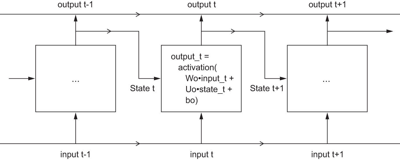
Note
In this example, the final output is a rank-2 tensor of shape (timesteps, output_features), where each timestep is the output of the loop at time t. Each timestep t in the output tensor contains information about timesteps 1 to t in the input sequence—about the entire past. For this reason, in many cases, we don’t need this full sequence of outputs; we just need the last output (output_t at the end of the loop), because it already contains information about the entire sequence.
13.3.2 A recurrent layer in Keras
The process we just naively implemented corresponds to an actual Keras layer: the SimpleRNN layer. There is one minor difference: SimpleRNN processes batches of sequences, like all other Keras layers, not a single sequence as in the simple example. This means it takes inputs of shape (batch_size, timesteps, input_features), rather than (timesteps, input_features). When specifying the shape argument of our initial keras_input(), note that we can set the timesteps entry to NA, which enables our network to process sequences of arbitrary length.
num_features <- 14
inputs <- keras_input(shape = c(NA, num_features))
outputs <- inputs |> layer_simple_rnn(16)
This is especially useful if your model is meant to process sequences of variable length. However, if all of your sequences have the same length, we recommend specifying a complete input shape: doing so enables print(model) to display output length information, which is always nice, and it can unlock some performance optimizations (see the sidebar “On RNN runtime performance”).
All recurrent layers in Keras (SimpleRNN, LSTM, and GRU) can be run in two different modes: they can return either full sequences of successive outputs for each timestep (a rank-3 tensor of shape (batch_size, timesteps, output_features)) or only the last output for each input sequence (a rank-2 tensor of shape (batch_size, output_features)). These two modes are controlled by the return_sequences constructor argument. Let’s look at an example that uses SimpleRNN and returns only the output at the last timestep.
num_features <- 14
steps <- 120
inputs <- keras_input(shape = c(steps, num_features))
1outputs <- inputs |> layer_simple_rnn(16, return_sequences = FALSE)
op_shape(outputs)- 1
- Note that return_sequences=FALSE is the default.
shape(NA, 16)The following example returns the full output sequence.
num_features <- 14
steps <- 120
inputs <- keras_input(shape = c(steps, num_features))
1outputs <- inputs |> layer_simple_rnn(16, return_sequences = TRUE)
op_shape(outputs)- 1
-
Sets return_sequences to
TRUE
shape(NA, 120, 16)It’s sometimes useful to stack several recurrent layers one after the other to increase the representational power of a network. In such a setup, we have to get all of the intermediate layers to return the full sequence of outputs.
inputs <- keras_input(shape = c(steps, num_features))
outputs <- inputs |>
  layer_simple_rnn(16, return_sequences = TRUE) |>
  layer_simple_rnn(16, return_sequences = TRUE) |>
  layer_simple_rnn(16)
Note that you’ll rarely work with the SimpleRNN layer. It’s generally too simplistic to be of real use. In particular, SimpleRNN has a major problem: although it should theoretically be able to retain at time t information about inputs seen many timesteps before, in practice, such long-term dependencies prove impossible to learn. This is due to the vanishing gradient problem, an effect that is similar to what is observed with nonrecurrent networks (feedforward networks) that are many layers deep: as we keep adding layers to a network, the network eventually becomes untrainable. The theoretical reasons for this effect were studied by Sepp Hochreiter, Jürgen Schmidhuber, and Yoshua Bengio in the early 1990s.2
Fortunately, SimpleRNN isn’t the only recurrent layer available in Keras. There are two others, LSTM and GRU, which were designed to address these problems.
Let’s consider the LSTM layer. The underlying LSTM algorithm was developed by Hochreiter and Schmidhuber in 1997 (“Long Short-Term Memory,” Neural Computation 9, no. 8 [1997]). It was the culmination of their research on the vanishing gradient problem.
This layer is a variant of the SimpleRNN layer; it adds a way to carry information across many timesteps. Imagine a conveyor belt running parallel to the sequence we’re processing. Information from the sequence can jump onto the conveyor belt at any point, be transported to a later timestep, and jump off, intact, when we need it. This is essentially what LSTM does: it saves information for later, thus preventing older signals from gradually vanishing during processing. This should remind you of residual connections, which you learned about in chapter 9: it’s pretty much the same idea.
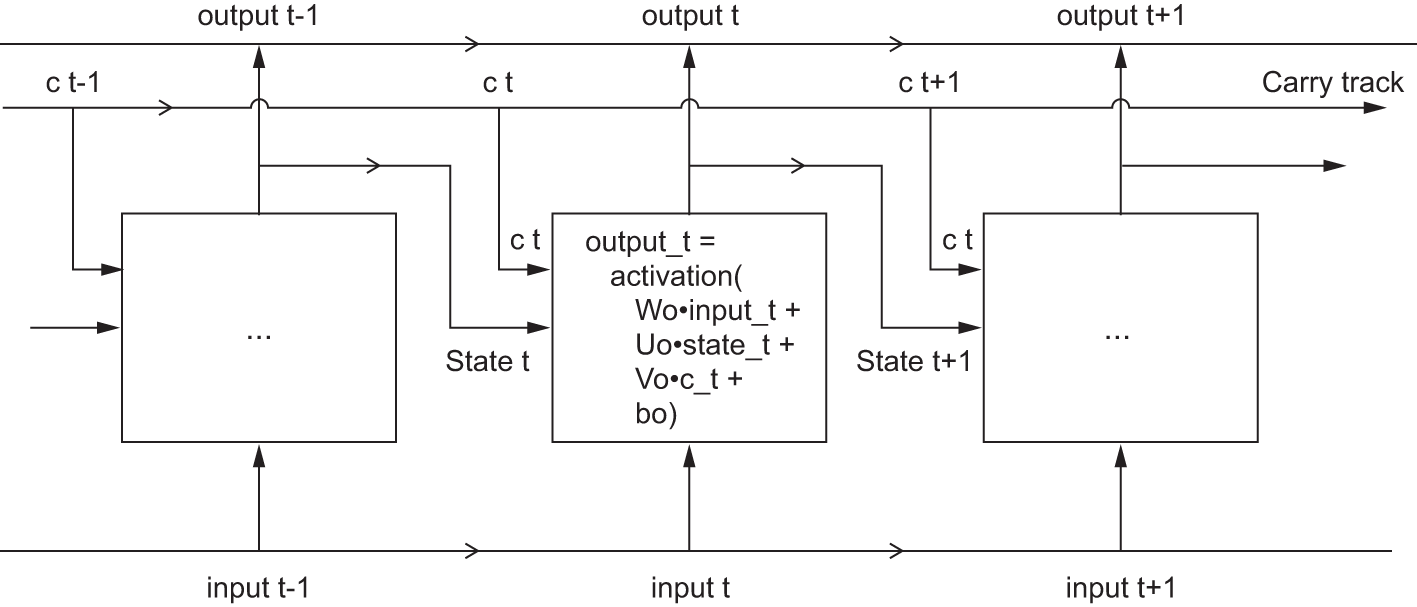
To understand this process in detail, let’s start from the SimpleRNN cell shown in figure 13.7. Because we’ll have a lot of weight matrices, we’ll index the W and U matrices in the cell with the letter o (Wo and Uo) for output.
Let’s add to this picture an additional data flow that carries information across timesteps. Call its values at different timesteps c_t, where c stands for carry. This information will have the following effect on the cell: it will be combined with the input connection and the recurrent connection (via a dense transformation: a dot product with a weight matrix followed by a bias add and the application of an activation function), and it will affect the state being sent to the next timestep (via an activation function and a multiplication operation). Conceptually, the carry dataflow is a way to modulate the next output and the next state (see figure 13.8). Simple so far.
Now comes the subtlety: the way the next value of the carry dataflow is computed. It involves three distinct transformations. All three have the form of a SimpleRNN cell:
y <- activation( (state_t %*% U) + (input_t %*% W) + b )But all three transformations have their own weight matrices, which we’ll index with the letters i, f, and k. Here’s what we have so far (it may seem a bit arbitrary, but bear with us).
output_t <-
activation((state_t %*% Uo) + (input_t %*% Wo) + (c_t %*% Vo) + bo)
i_t <- activation((state_t %*% Ui) + (input_t %*% Wi) + bi)
f_t <- activation((state_t %*% Uf) + (input_t %*% Wf) + bf)
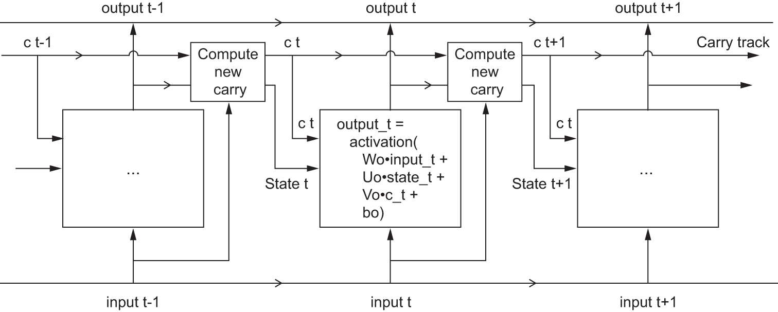
k_t <- activation((state_t %*% Uk) + (input_t %*% Wk) + bk)We obtain the new carry state (the next c_t) by combining i_t, f_t, and k_t.
c_t+1 = i_t * k_t + c_t * f_tAdd this as shown in figure 13.9. And that’s it. Not so complicated—merely a tad complex.
LSTMIf you want to get philosophical, you can interpret what each of these operations is meant to do. For instance, you can say that multiplying c_t and f_t is a way to deliberately forget irrelevant information in the carry dataflow. Meanwhile, i_t and k_t provide information about the present, updating the carry track with new information. But at the end of the day, these interpretations don’t mean much because what these operations actually do is determined by the contents of the weights parameterizing them, and the weights are learned in an end-to-end fashion, starting over with each training round, making it impossible to credit this or that operation with a specific purpose. The specification of an RNN cell (as just described) determines our hypothesis space—the space in which we’ll search for a good model configuration during training—but it doesn’t determine what the cell does; that is up to the cell weights. The same cell with different weights can be doing very different things. So the combination of operations making up an RNN cell is better interpreted as a set of constraints on our search, not as a design in an engineering sense.
Arguably, the choice of such constraints—the question of how to implement RNN cells—is better left to optimization algorithms (like genetic algorithms or reinforcement learning processes) than to human engineers. In the future, that’s how we’ll build our models. In summary, you don’t need to understand anything about the specific architecture of an LSTM cell; as a human, it shouldn’t be your job to understand it. Just keep in mind what the LSTM cell is meant to do: allow past information to be reinjected at a later time, thus fighting the vanishing-gradient problem.
13.3.3 Getting the most out of RNNs
By this point, you’ve learned the following:
- What RNNs are and how they work
- What an LSTM is and why it works better on long sequences than a naive RNN
- How to use Keras RNN layers to process sequence data
Next, we’ll review a number of more advanced features of RNNs, which can help you get the most out of your deep learning sequence models. By the end of the section, you’ll know most of what there is to know about using recurrent networks with Keras.
We’ll cover the following:
- Recurrent dropout—This is a variant of dropout, used to fight overfitting in recurrent layers.
- Stacking recurrent layers—This increases the representational power of the model (at the cost of higher computational loads).
- Bidirectional recurrent layers—These present the same information to a recurrent network in different ways, increasing accuracy and mitigating forgetting problems.
We’ll use these techniques to refine our temperature-forecasting RNN.
13.3.4 Using recurrent dropout to fight overfitting
Let’s go back to the LSTM-based model we used earlier in the chapter: our first model that could beat the common-sense baseline. If you look at the training and validation curves, it’s evident that the model is quickly overfitting, despite having very few units: the training and validation losses start to diverge considerably after a few epochs. You’re already familiar with a classic technique for fighting this phenomenon: dropout, which randomly zeros out input units of a layer to break happenstance correlations in the training data that the layer is exposed to. But how to correctly apply dropout in recurrent networks isn’t a trivial question.
It has long been known that applying dropout before a recurrent layer hinders learning rather than helping with regularization. In 2015, Yarin Gal, as part of his PhD thesis on Bayesian deep learning3 determined the proper way to use dropout with a recurrent network: the same dropout mask (the same pattern of dropped units) should be applied at every timestep, instead of a dropout mask that varies randomly from timestep to timestep. What’s more, to regularize the representations formed by the recurrent gates of layers such as GRU and LSTM, a temporally constant dropout mask should be applied to the inner recurrent activations of the layer (a recurrent dropout mask). Using the same dropout mask at every timestep allows the network to properly propagate its learning error through time; a temporally random dropout mask would disrupt this error signal and be harmful to the learning process.
Gal did his research using Keras and helped build this mechanism directly into Keras recurrent layers. Every recurrent layer in Keras has two dropout-related arguments: dropout, a float specifying the dropout rate for input units of the layer, and recurrent_dropout, specifying the dropout rate of the recurrent units. Let’s add recurrent dropout to the LSTM layer of our first LSTM example and see how doing so affects overfitting.
Thanks to dropout, we won’t need to rely as much on network size for regularization, so we’ll use an LSTM layer with twice as many units, which should hopefully be more expressive (without dropout, this network would have started overfitting right away—try it). Because networks being regularized with dropout always take much longer to fully converge, we’ll train the model for five times as many epochs.
inputs <- keras_input(shape = c(sequence_length, ncol_input_data))
outputs <- inputs |>
  layer_lstm(32, recurrent_dropout = 0.25) |>
1  layer_dropout(0.5) |>
  layer_dense(1)
model <- keras_model(inputs, outputs)

callbacks = list(
  callback_model_checkpoint("jena_lstm_dropout.keras", save_best_only = TRUE)
)

compile(model, optimizer = "adam", loss = "mse", metrics = "mae")- 1
-
To regularize the
Denselayer, we also add aDropoutlayer after theLSTM.
history <- model |> fit(
train_dataset,
epochs = 50,
validation_data = val_dataset,
callbacks = callbacks
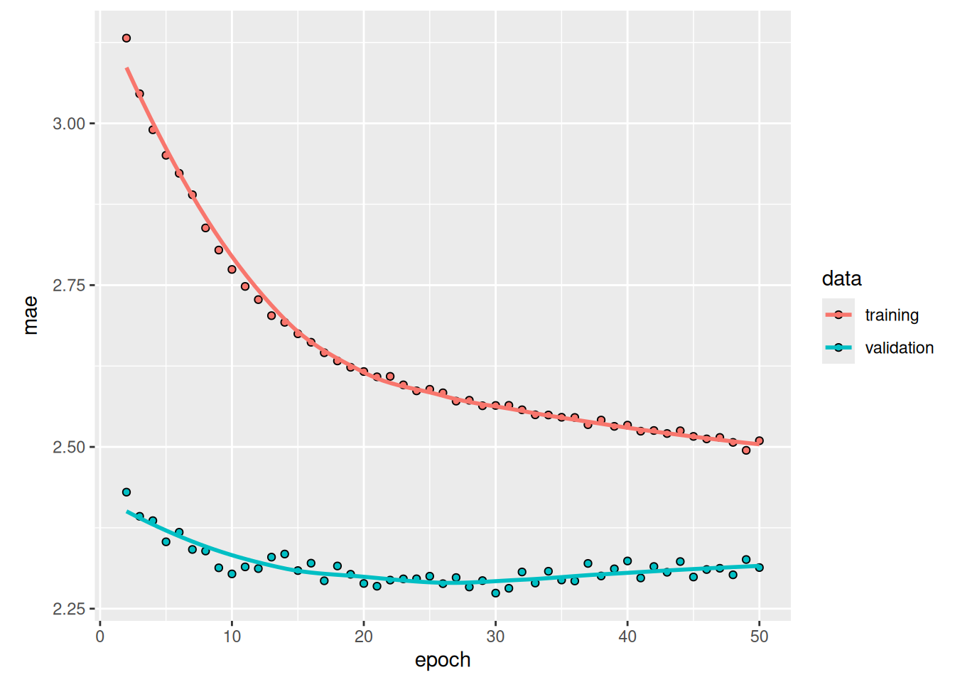
)Figure 13.10 shows the results. Success! We’re no longer overfitting during the first 20 epochs. We achieve a validation MAE as low as 2.27 degrees (7% improvement over the no-learning baseline) and a test MAE of 2.45 degrees (6.5% improvement over the baseline). Not too bad.
NoteOn RNN runtime performance
Recurrent models with very few parameters, like the ones in this chapter, tend to be significantly faster on a multicore CPU than on GPU because they only involve small matrix multiplications, and the chain of multiplications is not well parallelizable due to the presence of a for loop. But larger RNNs can greatly benefit from a GPU runtime.
When using a Keras LSTM or GRU layer on GPU with default keyword arguments, your layer will use a cuDNN kernel, a highly optimized, low-level, NVIDIA-provided implementation of the underlying algorithm (we mentioned those in the previous chapter). As usual, cuDNN kernels are a mixed blessing: they’re fast but inflexible—if you try doing anything not supported by the default kernel, you will suffer a dramatic slowdown, which more or less forces you to stick to what NVIDIA happens to provide. For instance, recurrent dropout isn’t supported by the LSTM and GRU cuDNN kernels, so adding it to your layers forces the runtime to fall back to the regular TensorFlow implementation, which is generally two to five times slower on GPU (even though its computational cost is the same).
As a way to speed up your RNN layer when you can’t use cuDNN, you can try unrolling it. Unrolling a for loop consists of removing the loop and simply inlining its content N times. In the case of the for loop of an RNN, unrolling can help TensorFlow optimize the underlying computation graph. However, it will also considerably increase the memory consumption of your RNN—as such, it’s only viable for relatively small sequences (around 100 steps or fewer). Also, you can only do this if the number of timesteps in the data is known in advance by the model (that is, if you pass a shape without any NA entries to your initial keras_input()). It works like this:
13.3.5 Stacking recurrent layers
Because we’re no longer overfitting but seem to have hit a performance bottleneck, we should consider increasing the capacity and expressive power of the network. Recall the description of the universal machine learning workflow: it’s generally a good idea to increase the capacity of our model until overfitting becomes the primary obstacle (assuming we’re already taking basic steps to mitigate overfitting, such as using dropout). As long as we aren’t overfitting too badly, we’re likely under capacity.
Increasing network capacity is typically done by increasing the number of units in the layers or adding more layers. Recurrent layer stacking is a classic way to build more powerful recurrent networks: for instance, not long ago, the Google Translate algorithm was powered by a stack of seven large LSTM layers—that’s huge.
To stack recurrent layers on top of each other in Keras, all intermediate layers should return their full sequence of outputs (a rank-3 tensor) rather than their output at the last timestep. As you’ve already learned, this is done by specifying return_sequences=TRUE.
In the following example, we’ll try a stack of two dropout-regularized recurrent layers. For a change, we’ll use gated recurrent unit (GRU) layers instead of LSTM (figure 13.11). A GRU is very similar to an LSTM—you can think of it as a slightly simpler, streamlined version of the LSTM architecture. It was introduced in 2014 by Kyunghyun Cho et al.4 just when recurrent networks were starting to gain interest in the then-tiny research community.
inputs <- keras_input(shape = c(sequence_length, ncol_input_data))
outputs <- inputs |>
  layer_gru(32, recurrent_dropout = 0.5, return_sequences = TRUE) |>
  layer_gru(32, recurrent_dropout = 0.5) |>
  layer_dropout(0.5) |>
  layer_dense(1)
model <- keras_model(inputs, outputs)

callbacks <- list(
  callback_model_checkpoint(
    "jena_stacked_gru_dropout.keras", save_best_only = TRUE
  )
)

model |> compile(optimizer = "adam", loss = "mse", metrics = "mae")
history <- model |> fit(
train_dataset,
epochs = 50,
validation_data = val_dataset,
callbacks = callbacks
)plot(history)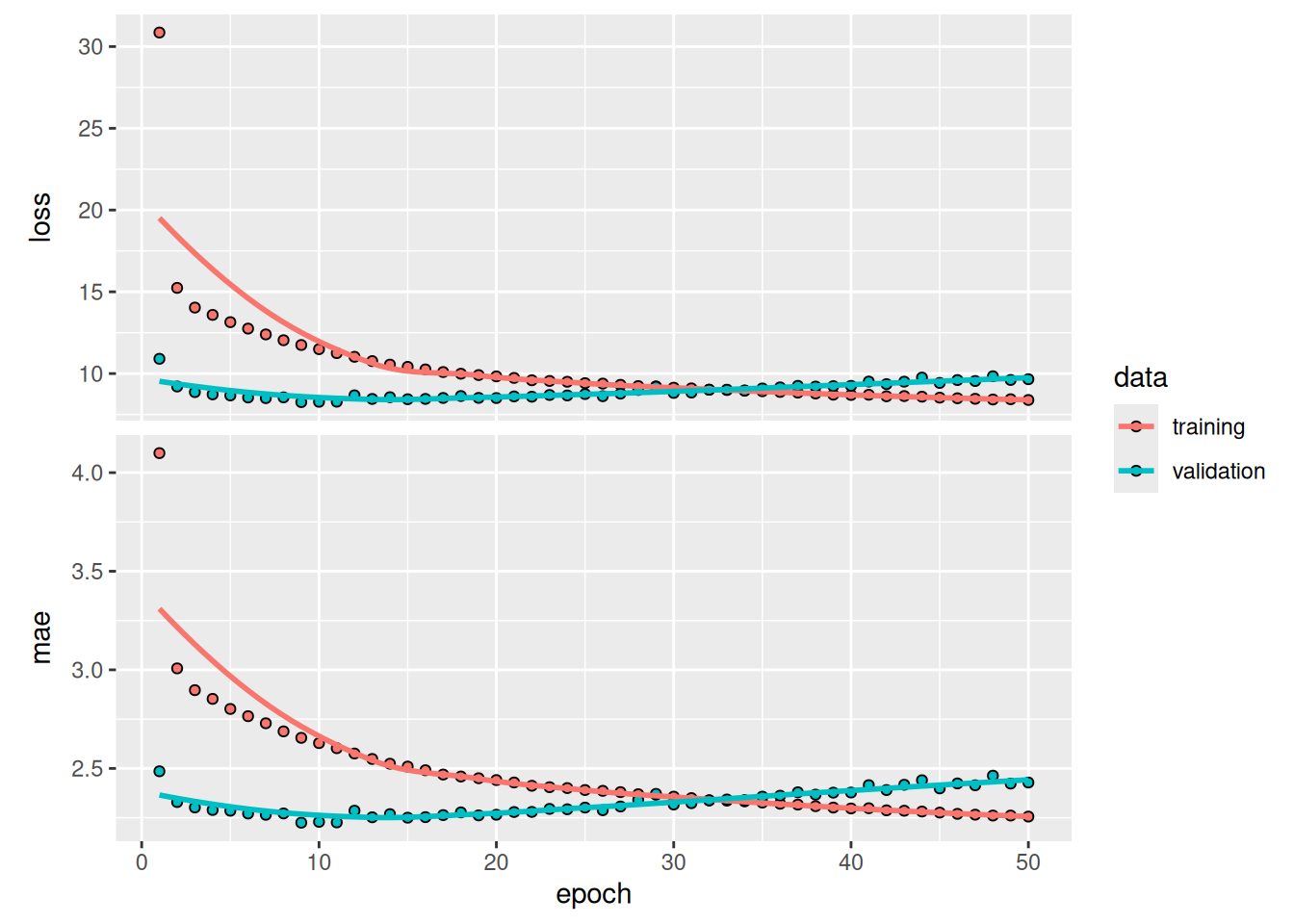
model <- load_model("jena_stacked_gru_dropout.keras")
sprintf("Test MAE: %.2f", evaluate(model, test_dataset)[["mae"]])
[1] "Test MAE: 2.40"Figure 13.12 shows the results. We achieve a test MAE of 2.40 degrees (about 8.3% improvement over the baseline). The added layer does improve the results a bit, although not dramatically. We may be seeing diminishing returns from increasing network capacity at this point.
13.3.6 Using bidirectional RNNs
The last technique introduced in this section is called bidirectional RNNs. A bidirectional RNN is a common RNN variant that can offer greater performance than a regular RNN on certain tasks. It’s frequently used in natural language processing—you could call it the Swiss Army knife of deep learning for natural language processing.
RNNs are notably order-dependent: they process the timesteps of their input sequences in order, and shuffling or reversing the timesteps can completely change the representations the RNN extracts from the sequence. This is precisely the reason they perform well on problems where order is meaningful, such as the temperature-forecasting problem. A bidirectional RNN exploits the order sensitivity of RNNs: it consists of using two regular RNNs, such as the GRU and LSTM layers you’re already familiar with, each of which processes the input sequence in one direction (chronologically and antichronologically), and then merging their representations. By processing a sequence both ways, a bidirectional RNN can catch patterns that may be overlooked by a unidirectional RNN.
Remarkably, the fact that the RNN layers in this section have processed sequences in chronological order (older timesteps first) may have been an arbitrary decision. At least, it’s a decision we made no attempt to question so far. Could the RNNs have performed well enough if they processed input sequences in antichronological order, for instance (newer timesteps first)? Let’s try this in practice and see what happens. All we need to do is write a variant of the data generator in which the input sequences are reverted along the time dimension.
To do this, we simply transform the dataset with dataset_map(), like this:
dataset <- dataset |>
  dataset_map(\(samples, targets) {
    list(samples@r[, NA:NA:-1, ], targets)
  })
When training the same LSTM-based model that we used in the first experiment in this section, such a reversed-order LSTM strongly underperforms even the common-sense baseline. This indicates that in this case, chronological processing is important to the success of the approach. This makes perfect sense: the underlying LSTM layer will typically be better at remembering the recent past than the distant past, and, naturally, the more recent weather data points are more predictive than older data points for the problem (that’s what makes the common-sense baseline fairly strong). Thus, the chronological version of the layer is bound to outperform the reversed-order version.
However, this isn’t true for many other problems, including natural language: intuitively, the importance of a word in understanding a sentence isn’t strongly dependent on its position in the sentence. On text data, reversed-order processing works just as well as chronological processing—we can read text backward just fine (try it!). Although word order does matter in understanding language, which order we use isn’t crucial.
Importantly, an RNN trained on reversed sequences will learn different representations than one trained on the original sequences, much as we would have different mental models if time flowed backward in the real world—if we lived a life where we died on our first day and were born on our last day. In machine learning, representations that are different yet useful are always worth exploiting, and the more they differ, the better: they offer a new angle from which to look at our data, capturing aspects of the data that were missed by other approaches, and thus they can help boost performance on a task. This is the intuition behind ensembling, a concept we’ll explore in chapter 18.
A bidirectional RNN exploits this idea to improve on the performance of chronological-order RNNs. It looks at its input sequence both ways (see figure 13.13), obtaining potentially richer representations and capturing patterns that may have been missed by the chronological-order version alone.
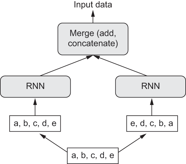
To instantiate a bidirectional RNN in Keras, we use the Bidirectional layer, which takes as its first argument a recurrent layer instance. Bidirectional creates a second, separate instance of this recurrent layer and uses one instance for processing the input sequences in chronological order and the other instance for processing the input sequences in reverse order. We can try it on our temperature forecasting task (figure 13.14).
inputs <- keras_input(shape = c(sequence_length, ncol_input_data))
outputs <- inputs |>
  layer_bidirectional(layer_lstm(units = 16)) |>
  layer_dense(1)
model <- keras_model(inputs, outputs)

model |> compile(optimizer = "adam", loss = "mse", metrics = "mae")
history <- model |> fit(
train_dataset,
epochs = 10,
validation_data = val_dataset
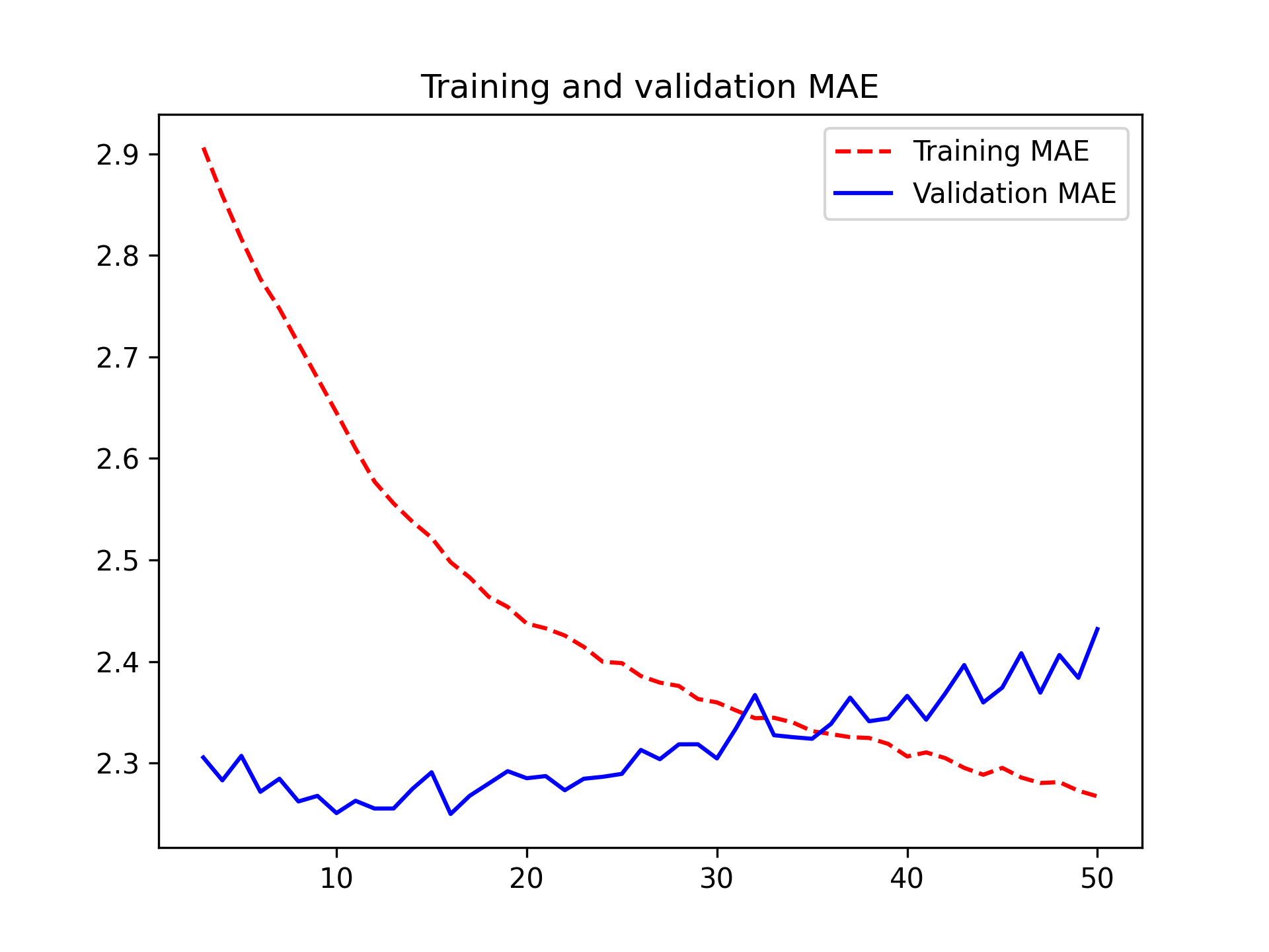
)plot(history)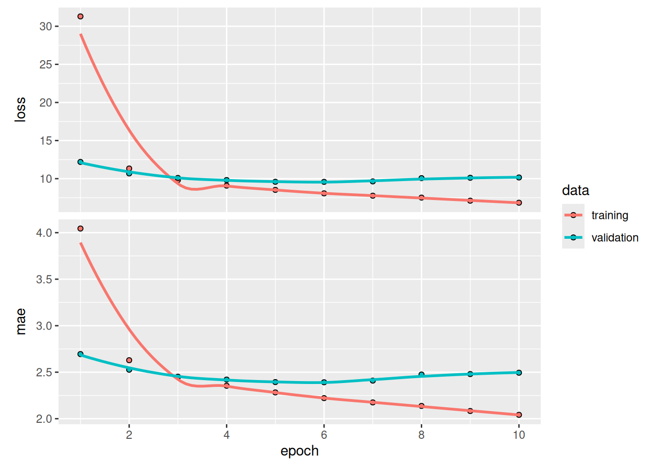
You’ll find that it doesn’t perform as well as the plain LSTM layer. It’s easy to understand why: all the predictive capacity must come from the chronological half of the network because the antichronological half is known to be severely underperforming on this task (again, because the recent past matters much more than the distant past in this case). At the same time, the presence of the antichronological half doubles the network’s capacity and causes it to start overfitting much earlier.
However, bidirectional RNNs are a great fit for text data—or any other kind of data for which order matters, but which order we use doesn’t matter. In fact, for a while in 2016, bidirectional LSTMs were considered the state of the art on many natural language processing tasks (before the rise of the Transformer architecture, which you will learn about in the next chapter).
13.4 Going even further
There are many other things you could try to improve performance on the temperature-forecasting problem:
- Adjust the number of units in each recurrent layer in the stacked setup, as well as the amount of dropout. The current choices are largely arbitrary and thus probably suboptimal.
- Adjust the learning rate used by the
Adamoptimizer, or try a different optimizer. - Try using a stack of
Denselayers as the regressor on top of the recurrent layer, instead of a singleDenselayer. - Improve the input to the model: try using longer or shorter sequences, or a different sampling rate, or start doing feature engineering.
As always, deep learning is more of an art than a science. We can provide guidelines that suggest what is likely to work or not work on a given problem, but ultimately, every dataset is unique; you’ll have to evaluate different strategies empirically. There is currently no theory that will tell you in advance precisely what you should do to optimally solve a problem. You must iterate.
In our experience, improving on the no-learning baseline by about 10% is likely the best you can do with this dataset. That isn’t great, but these results make sense: although near-future weather is highly predictable if you have access to data from a wide grid of different locations, it’s not very predictable if you only have measurements from a single location. The evolution of the weather where you are depends on current weather patterns in surrounding locations.
NoteMarkets and machine learning
Some readers are bound to want to take the techniques we’ve introduced here and try them on the problem of forecasting the future price of securities on the stock market (or currency exchange rates, and so on). However, markets have very different statistical characteristics from natural phenomena such as weather patterns. When it comes to markets, past performance is not a good predictor of future returns—looking in the rear-view mirror is a bad way to drive. Machine learning, on the other hand, is applicable to datasets where the past is a good predictor of the future, like weather, electricity consumption, or foot traffic at a store.
Remember that all trading is fundamentally information arbitrage: gaining an advantage by using data or insights that other market participants are missing. Trying to use well-known machine learning techniques and publicly available data to beat the markets is effectively a dead end, because you won’t have any information advantage compared to everyone else. You’re likely to waste your time and resources with nothing to show for it.
13.5 Summary
As you first learned in chapter 6, when approaching a new problem, it’s good to first establish common-sense baselines for your metric of choice. If you don’t have a baseline to beat, you can’t tell whether you’re making real progress.
Try simple models before expensive ones, to justify the additional expense. Sometimes a simple model will turn out to be your best option.
When you have data where ordering matters—in particular, timeseries data— recurrent networks are a great fit and easily outperform models that first flatten the temporal data. The two essential RNN layers available in Keras are the
LSTMlayer and theGRUlayer.To use dropout with recurrent networks, you should use a time-constant dropout mask and recurrent dropout mask. These are built into Keras recurrent layers, so all you have to do is use the
recurrent_dropoutarguments of recurrent layers.Stacked RNNs provide more representational power than a single RNN layer. They’re also much more expensive and thus not always worth it. Although they offer clear gains on complex problems (such as machine translation), they may not always be relevant to smaller, simpler problems.
Adam Erickson and Olaf Kolle, https://www.bgc-jena.mpg.de/wetter↩︎
See, for example, Bengio, Patrice Simard, and Paolo Frasconi, “Learning Long-Term Dependencies with Gradient Descent Is Difficult,” IEEE Transactions on Neural Networks 5, no. 2 [1994]↩︎
Uncertainty in Deep Learning, https://www.cs.ox.ac.uk/people/yarin.gal/website/blog_2248.html↩︎
“On the Properties of Neural Machine Translation: Encoder-Decoder Approaches,” https://arxiv.org/abs/1409.1259↩︎