

library(keras3)
zipfile <-
"https://hf.co/datasets/mattdangerw/mini-c4/resolve/main/mini-c4.zip" |>
get_file(origin = _)
unzip(zipfile, exdir = ".")
extract_dir <- fs::path("./mini-c4")16 Text generation
This chapter covers
- A brief history of generative modeling
- Training a miniature GPT model from scratch
- Using a pretrained Transformer model to build a chatbot
- Building a multimodal model that can describe images in natural language
In 2014, the idea that, in a not-so-distant future, most of the cultural content we consume would be created with substantial help from AI was met with utter disbelief, even among long-time machine learning practitioners. Fast-forward a decade, and that disbelief has receded at an incredible speed. Generative AI tools are now common additions to word processors, image editors, and development environments. Prestigious awards are going out to literature and art created with generative models—causing considerable controversy and debate. 1 It no longer feels like science fiction to consider a world where AI and artistic endeavors are often intertwined.
In any practical sense, AI is nowhere close to rivaling human screenwriters, painters, or composers. But replacing humans need not, and should not, be the point. In many fields, but especially in creative ones, people will use AI to augment their capabilities—more augmented intelligence than artificial intelligence.
Much of artistic creation consists of pattern recognition and technical skill. Our perceptual modalities, language, and artwork all have statistical structure, and deep learning models excel at learning this structure. Machine learning models can learn the statistical latent spaces of images, music, and stories, and they can then sample from these spaces, creating new artworks with characteristics similar to those the model has seen in its training data. Such sampling is hardly an act of artistic creation in itself—it’s a mere mathematical operation. Only our interpretation, as human spectators, gives meaning to what the model generates. But in the hands of a skilled artist, algorithmic generation can be steered to become meaningful—and beautiful. Latent space sampling can become a brush that empowers the artist, augments our creative affordances, and expands the space of what we can imagine. It can even make artistic creation more accessible by eliminating the need for technical skill and practice, setting up a new medium of pure expression, factoring art apart from craft.
Iannis Xenakis, a visionary pioneer of electronic and algorithmic music, beautifully expressed this same idea in the 1960s, in the context of the application of automation technology to music composition2:
Freed from tedious calculations, the composer is able to devote himself to the general problems that the new musical form poses and to explore the nooks and crannies of this form while modifying the values of the input data. For example, he may test all instrumental combinations from soloists to chamber orchestras, to large orchestras. With the aid of electronic computers the composer becomes a sort of pilot: he presses the buttons, introduces coordinates, and supervises the controls of a cosmic vessel sailing in the space of sound, across sonic constellations and galaxies that he could formerly glimpse only as a distant dream.
Figure 16.1 shows an image generated with the generative image software Midjourney.

The potential for generative AI extends well beyond artistic endeavors. In many professions, people create content where pattern recognition is even more apparent: think of summarizing large documents, transcribing speech, editing for typos, or flagging common mistakes in code. These rote tasks play directly to the strengths of deep learning approaches. There is a lot to consider regarding how we choose to deploy AI in the workplace—with real societal implications.
In this chapter and the next, we will explore the potential of deep learning to assist with creation. We will learn to curate latent spaces in text and image domains and pull new content from these spaces. We will start with text, scaling up the idea of a language model we first worked with in the last chapter. These large language models (LLMs) are behind digital assistants like ChatGPT and a quickly growing list of real-world applications.
16.1 A brief history of sequence generation
Until recently, the idea of generating sequences from a model was a niche subtopic within machine learning; generative recurrent networks only began to hit the mainstream in 2016. However, these techniques have a fairly long history, starting with the development of the LSTM algorithm in 1997.
In 2002, Douglas Eck applied LSTM to music generation for the first time, with promising results. Eck became a researcher at Google Brain, and in 2016, he formed a new research group called Magenta that focused on applying modern deep learning techniques to produce engaging music. Sometimes good ideas take 15 years to get started.
In the late 2000s and early 2010s, Alex Graves pioneered the use of recurrent networks for new types of sequence data generation. In particular, some see his 2013 work on applying recurrent mixture density networks to generate human-like handwriting using timeseries of pen positions as a turning point. Graves left a commented-out remark hidden in a 2013 LaTeX file uploaded to the preprint server arXiv: “Generating sequential data is the closest computers get to dreaming.” This work and the notion of machines that dream were significant inspirations for the creation of Keras.
In 2018, a year after the “Attention Is All You Need” paper we discussed in the last chapter, a group of researchers at an organization called OpenAI put out a new paper, “Improving Language Understanding by Generative Pre-Training” (Alec Radford, Karthik Narasimhan, Tim Salimans, and Ilya Sutskever, https://mng.bz/GweD). They combined a few ingredients:
- Unsupervised pretraining of a language model—essentially, training a model to “guess the next token” in a sequence, as we did with our Shakespeare generator in chapter 15
- The Transformer architecture
- Textual data on various topics via thousands of self-published books
The authors showed that such a pretrained model could be fine-tuned to achieve state-of-the-art performance on a wide array of text classification tasks, from gauging the similarity of two sentences to answering a multiple-choice question. They called the pretrained model GPT, short for Generative Pretrained Transformer.
GPT didn’t come with any modeling or training advancements. What was interesting about the results was that such a general training setup could beat out more involved techniques across a number of tasks. There was no complex text normalization, no need to customize the model architecture or training data per benchmark, just a lot of pretraining data and compute.
In the following years, OpenAI set about scaling this idea with a single-minded focus. The model architecture changed only slightly. Over four years, OpenAI released three versions of GPT, scaling up as follows:
- Released in 2018, GPT-1 had 117 million parameters and was trained on 1 billion tokens.
- Released in 2019, GPT-2 had 1.5 billion parameters and was trained on more than 10 billion tokens.
- Released in 2020, GPT-3 had 175 billion parameters and was trained on somewhere around half a trillion tokens.
The language modeling setup enabled each of these models to generate text, and the developers at OpenAI noticed that with each leap in scale, the quality of this generative output shot up substantially.
With GPT-1, the model’s generative capabilities were mostly a by-product of its pretraining and not the primary focus. They evaluated the model by fine-tuning it with an extra Dense layer for classification, as we did with RoBERTa in the last chapter.
With GPT-2, the authors noticed that they could prompt the model with a few examples of a task and generate quality output without any fine-tuning. For instance, they could prompt the model with the following to receive a French translation of the word cheese:
Translate English to French:

sea otter => loutre de mer
peppermint => menthe poivrée
plush giraffe => peluche girafe
cheese =>
This type of setup is called few-shot learning, where we attempt to teach a model a new problem with only a handful of supervised examples—too few for standard gradient descent.
With GPT-3, examples weren’t always necessary. The authors could prompt the model with a simple text description of the problem and the input and often get quality results:
Translate English to French:

cheese =>
GPT-3 was still plagued by fundamental problems that have yet to be solved. LLMs “hallucinate” often: their output can veer from accurate to completely false with zero indication. They’re extremely sensitive to prompt phrasing, with seemingly minor prompt rewording triggering large jumps up or down in performance. And they cannot adapt to problems that weren’t extensively featured in their training data.
However, the generative output from GPT-3 was good enough that the model became the basis for ChatGPT—the first widespread, consumer-facing generative model. In the months and years since, ChatGPT has sparked a deluge of investment and interest in building LLMs and finding new use cases for them. In the next section, we will make a miniature GPT model of our own to better understand how such a model works, what it can do, and where it fails.
16.2 Training a mini-GPT
To begin pretraining our mini-GPT, we will need a lot of text data. GPT-1 used a dataset called BooksCorpus, which contained a number of free, self-published books that were added to the dataset without the explicit permission of the authors. The dataset has since been taken down by its publishers.
We will use a more recent pretraining dataset called the “Colossal Clean Crawled Corpus” (C4), released by Google in 2020. At 750 GB, it’s far bigger than we could reasonably train on for a book example, so we will use less than 1% of the overall corpus. Let’s start by downloading and extracting our data:
NoteRunning the code in this chapter
Generative language models are big and take a lot of compute to run. Although we’ve taken pains to make the code in this chapter accessible, this is still the most compute-intensive chapter in this book.
If you’d like, you can run everything on the free Colab GPU runtime (a T4 GPU as of this writing), but be prepared to wait! This mini-GPT example will take about 6 hours to train, and you will need to restart the Colab runtime in the middle of the notebook to free up GPU memory before loading a larger pretrained model. A larger GPU will make quicker work of these examples; we developed this example on an A100, which can run this chapter’s code end-to-end in a little over an hour.
You can always read through the expensive fit() calls and edit down the number of training steps for quick experimentation. And if you are running this a few years down the line, there is a good chance these examples are mere child’s play with modern hardware!
We have 50 shards of text data, each with about 75 MB of raw text. Each line contains a document in the crawl with newlines escaped. Let’s look at a document in our first shard:
library(stringr)

fs::path(extract_dir, "shard0.txt") |> readLines(n = 1) |>
  str_replace_all(r"(\\n)", "\n") |> str_sub(1, 100) |> cat()
Beginners BBQ Class Taking Place in Missoula!
Do you want to get better at making delicious BBQ? YouWe will need to preprocess a lot of data to run pretraining for an LLM, even a miniature one like the one we are training. Using a fast tokenization routine to preprocess our source documents into integer tokens can simplify our lives.
We will use SentencePiece, a library for subword tokenization of text data. The actual tokenization technique is the same as the byte-pair encoding tokenization we built ourselves in chapter 14, but the library is written in C++ for speed and adds a detokenize() function that will reverse integers to strings and join them together. We will use a premade vocabulary with 32,000 vocabulary terms stored in a particular format needed by the SentencePiece library.
As in the last chapter, we can use the KerasHub library to access some extra functions for working with large language models. KerasHub wraps the SentencePiece library as a Keras layer. Let’s try it out.
py_require("keras_hub")
keras_hub <- import("keras_hub")

vocabulary_file <- get_file(
  origin = "https://hf.co/mattdangerw/spiece/resolve/main/vocabulary.proto"
)
tokenizer <- keras_hub$tokenizers$SentencePieceTokenizer(vocabulary_file)
We can use this tokenizer to map from text to int sequences bidirectionally:
(tokenized <- tokenizer$tokenize("The quick brown fox."))Array([ 450, 4996, 17354, 1701, 29916, 29889], dtype=int32)tokenizer$detokenize(tokenized)[1] "The quick brown fox."
NoteTraining SentencePiece (optional)
If you’d like to train a SentencePiece vocabulary yourself from the mini‑C4 shards, you could do it like this. This uses the sentencepiece Python package from R via reticulate and writes a small tokenizer model (mini_gpt.model, mini_gpt.vocab). Run it in a fresh/standalone R session to avoid environment conflicts:
library(fs)
library(readr)
library(purrr)
library(stringr)
library(reticulate)
py_require("sentencepiece")
spm <- import("sentencepiece")

tmp_dir <- path_temp("spm_corpus")
dir_create(tmp_dir)

files <- Sys.glob("./mini-c4/*.txt")
new_files <- path(tmp_dir, basename(files))
files <- map2_chr(files, new_files, \(f, f2) {
  f |>
    read_file() |>
    str_replace_all(r"(\\n)", "\n") |>
    write_file(f2)
  f2
  }, .progress = TRUE)

spm$SentencePieceTrainer$train(
  input = files |> str_flatten(","),
  model_prefix = "mini_gpt",
  vocab_size = 2048,
  input_sentence_size = 10000,
  max_sentence_length = 50000,
  shuffle_input_sentence = TRUE
)
You could then load the produced mini_gpt.model file the same way:
mini_tokenizer <-
  keras_hub$tokenizers$SentencePieceTokenizer("mini_gpt.model")
mini_tokenizer$tokenize("The quick brown fox.")
To keep things simple, we’ll use a larger pretrained SentencePiece vocabulary you can download directly.
Let’s use this layer to tokenize our input text and then use tf.data to window our input into sequences of length 256. When training GPT, the developers chose to keep things simple and make no attempt to keep document boundaries from occurring in the middle of a sample. Instead, they marked a document boundary with a special <|endoftext|> token. We will do the same here. Once again, we will use tf.data for the input data pipeline and train with any backend.
We will load each file shard individually and interleave the output data into a single dataset. This keeps our data loading fast, and we don’t need to worry about text lining up across sample boundaries—each is independent. With interleaving, each processor on our CPU can read and tokenize a separate file simultaneously.
library(tfdatasets, exclude = "shape")
library(tensorflow, exclude = c("shape", "set_random_seed"))

batch_size <- 128
sequence_length <- 256
suffix <- tf$constant(
  tokenizer$token_to_id("<|endoftext|>"),
  shape = shape(1L)
)

files <- dir_ls(extract_dir, glob = "*.txt")

read_file <- function(filename) {
  text_line_dataset(filename) |>
1    dataset_map(\(x) tf$strings$regex_replace(x, "\\\\n", "\n")) |>
2    dataset_map(tokenizer, num_parallel_calls = 8) |>
3    dataset_map(\(x) tf$concat(list(x, suffix), -1L))
}


ds <- tensor_slices_dataset(files) |>
  dataset_interleave(read_file, cycle_length = 32,
4                     num_parallel_calls = 32) |>
5  dataset_rebatch(sequence_length + 1, drop_remainder = TRUE)  |>
6  dataset_map(\(x) list(x@r[NA:-2], x@r[2:NA]),
              num_parallel_calls = 12) |>
  dataset_batch(batch_size) |>
dataset_prefetch(buffer_size = 8)- 1
- Restores newlines
- 2
- Tokenizes data
- 3
- Adds the <|endoftext|> token
- 4
- Combines our file shards into a single dataset
- 5
- Windows tokens into even samples of 256 tokens
- 6
- Splits labels, offset by one
As we first did in chapter 8, we will end our tf.data pipeline with a call to dataset_prefetch(). This will make sure we always have some batches loaded onto our GPU and ready for the model.
We have 29,373 batches. You can count this yourself if you like: the line dataset_reduce(ds, 0L, \(i, el) i + 1L) will iterate over the entire dataset and increment a counter. But simply tokenizing a dataset of this size will take a few minutes on a decently fast CPU.
At 128 samples per batch and 256 tokens per sample, this is just under a billion tokens of data. Let’s split off 500 batches as a quick validation set, and we are ready to start pretraining:
num_batches <- 29373
num_val_batches <- 500
num_train_batches <- num_batches - num_val_batches
val_ds <- ds |> dataset_take(num_val_batches) |> dataset_repeat()
train_ds <- ds |> dataset_skip(num_val_batches) |> dataset_repeat()
16.2.1 Building the model
The original GPT model simplifies the sequence-to-sequence Transformer you saw in the last chapter. Rather than take in a source and target sequence with an encoder and decoder, as we did for our translation model, the GPT approach does away with the encoder entirely and only uses the decoder. This means that information can only travel from left to right in a sequence.
This was an interesting bet on the side of the GPT developers. A decoder-only model can still handle sequence-to-sequence problems like question answering. However, rather than feeding in the question and answer as separate inputs, we must combine both into a single sequence to feed it to our model. So, unlike the original Transformer, the question tokens are not handled any differently from answer tokens. All tokens are embedded into the same latent space with the same set of parameters.
The other consequence of this approach is that the information flow is no longer bidirectional, even for input sequences. Given an input, such as “Where is the capital of France?”, the learned representation of the word “Where” cannot attend to the word “capital” or “France” in the attention layer. This limits the expressivity of the model but has a massive advantage in terms of simplicity of pretraining. We don’t need to curate datasets with pairs of inputs and outputs; everything can be a single sequence. We can train on any text we can find on the internet at a massive scale.
Let’s copy the TransformerDecoder from chapter 15 but remove the cross-attention layer, which allowed the decoder to attend to the encoder sequence. We will also make one minor change, adding dropout after the attention and feedforward blocks. In chapter 15, we used a single Transformer layer in our encoder and decoder, so we could get away with using only a single dropout layer at the end of our entire model. For our GPT model, we will stack quite a few layers, so adding dropout within each decoder layer is important to prevent overfitting.
layer_transformer_decoder <- new_layer_class(
  "TransformerDecoder",
  initialize = function(hidden_dim, intermediate_dim, num_heads) {
    super$initialize()
    key_dim <- hidden_dim %/% num_heads
    self$self_attention <- layer_multi_head_attention(
      num_heads = num_heads,
      key_dim = key_dim,
      dropout = 0.1
1    )
    self$self_attention_layernorm <- layer_layer_normalization()
    self$feed_forward_1 <- layer_dense(units = intermediate_dim,
2                                       activation = "relu")
    self$feed_forward_2 <- layer_dense(units = hidden_dim)
    self$feed_forward_layernorm <- layer_layer_normalization()
    self$dropout <- layer_dropout(rate = 0.1)
  },
  call = function(inputs) {
3    residual <- x <- inputs
    x <- self$self_attention(query = x, key = x, value = x,
                             use_causal_mask = TRUE)
    x <- x |> self$dropout()
    x <- x + residual
    x <- x |> self$self_attention_layernorm()

4    residual <- x
    x <- x |>
      self$feed_forward_1() |>
      self$feed_forward_2() |>
      self$dropout()
    x <- x + residual
    x <- x |> self$feed_forward_layernorm()

    x
  }
)- 1
- Self-attention layers.
- 2
- Feed-forward layers.
- 3
- Self-attention computation.
- 4
- Feed-forward computation.
Next, we can copy the PositionalEmbedding layer from chapter 15. Recall that this layer gives us a simple way to learn an embedding for each position in a sequence and combine that with our token embeddings.
There’s a neat trick we can employ here to save some GPU memory. The biggest weights in a Transformer model are the input token embeddings and the output Dense prediction layer because they deal with our vocabulary space. The token embedding weight has shape (vocab_size, hidden_dim) to embed every possible token. Our output projection has shape (hidden_dim, vocab_size) to make a floating-point prediction for every possible token.
We can actually tie these two weight matrices together. To compute our model’s final predictions, we will multiply our hidden states by the transpose of our token embedding matrix. You can think of our final projection as a “reverse embedding.” It maps from hidden space to token space, whereas an embedding maps from token space to hidden space. It turns out that using the same weights for this input and output projection is a good idea.
Adding this to our PositionalEmbedding is simple: we just add a reverse argument to the call method, which computes the projection by the transpose of the token embedding.
layer_positional_embedding <- new_layer_class(
  "PositionalEmbedding",
  initialize = function(sequence_length, input_dim, output_dim) {
    super$initialize()
    self$token_embeddings <- layer_embedding(
      input_dim = input_dim, output_dim = output_dim
    )
    self$position_embeddings <- layer_embedding(
      input_dim = sequence_length, output_dim = output_dim
    )
  },
  call = function(inputs, reverse = FALSE) {
    if (reverse) {
      token_embeddings <- self$token_embeddings$embeddings
1      return(inputs %*% t(token_embeddings))
    }
    .[.., sequence_length] <- op_shape(inputs)
    positions <-
      op_arange(0, sequence_length - 1, dtype = "int32") |>
      op_expand_dims(1)
    embedded_tokens <- self$token_embeddings(inputs)
    embedded_positions <- self$position_embeddings(positions)
    embedded_tokens + embedded_positions
  }
)- 1
-
%*%callsop_matmul(), andt()callsop_transpose().
Let’s build our model. We will stack eight decoder layers into a single “mini” GPT model.
We will also turn on a Keras setting called mixed precision to speed up training. This will allow Keras to run some of the model’s computations much faster by sacrificing some numerical fidelity. For now, this will remain a little mysterious, but a full explanation is waiting in chapter 18.
1config_set_dtype_policy("mixed_float16")
vocab_size <- tokenizer$vocabulary_size()
hidden_dim <- 512
intermediate_dim <- 2056
num_heads <- 8
num_layers <- 8

inputs <- keras_input(shape = c(NA), dtype = "int32", name = "inputs")
embedding <-
  layer_positional_embedding(, sequence_length, vocab_size, hidden_dim)

x <- inputs |>
  embedding() |>
  layer_layer_normalization()

for (i in seq_len(num_layers)) {
  x <- x |>
    layer_transformer_decoder(hidden_dim, intermediate_dim, num_heads)
}

outputs <- x |> embedding(reverse = TRUE)
mini_gpt <- keras_model(inputs, outputs)- 1
- Enables mixed precision (see chapter 18)
This model has 41 million parameters, which is large for models in this book but small compared to most LLMs today, which range from a couple of billion to trillions of parameters.
16.2.2 Pretraining the model
Training a large Transformer is famously finicky—the model is sensitive to initializations of parameters and choice of optimizer. When many Transformer layers are stacked, it is easy to suffer from exploding gradients, where parameters update too quickly and the loss function does not converge. A trick that works well is to linearly ease into a full learning rate over a number of warmup steps, so our initial updates to our model parameters are small. This is easy to implement in Keras with a LearningRateSchedule.
warmup_schedule <- new_learning_rate_schedule_class(
  classname = "WarmupSchedule",

  initialize = function() {
1    self$rate <- 2e-4
    self$warmup_steps <- 1000
  },

  call = function(step) {
    step <- step |> op_cast(dtype = "float32")
    scale <- op_minimum(step / self$warmup_steps, 1)
    self$rate * scale
  }
)- 1
- Peak learning rate
We can plot our learning rate over time to make sure it is what we expect (figure 16.2):
schedule <- warmup_schedule()
x <- seq(0, 5000, by = 10)
y <- sapply(x, \(step) as.array(schedule(step)))

par(mar = c(5, 7, 4, 2), bty = "n", ann = FALSE)
plot(x, y, type = "l", lwd = 2, panel.first = grid())
title(main = "Warmup Schedule", xlab = "Train Step")
title(ylab = "Learning Rate", line = 4.5)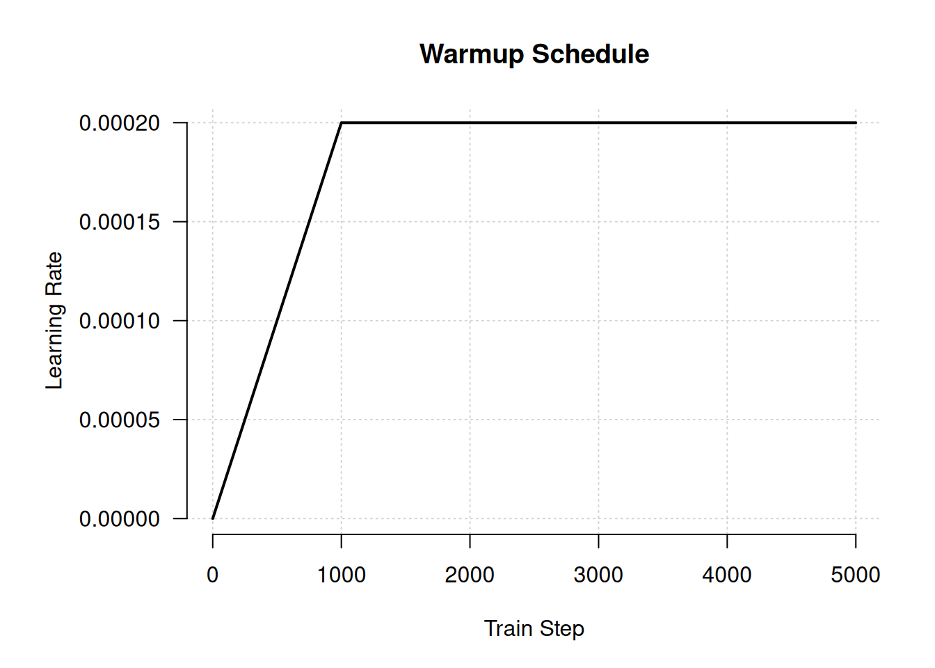
We will train our model using one pass over our 1 billion tokens, split across eight epochs so we can occasionally check our validation set loss and accuracy. We are training a miniature version of GPT, using 3 times fewer parameters than GPT-1 and 100 times fewer overall training steps. But despite this being two orders of magnitude cheaper to train than the smallest GPT model, this call to fit() will be the most computationally expensive training run in the entire book. If you are running the code as you read, take a breather!
num_epochs <- 8
1steps_per_epoch <- num_train_batches %/% num_epochs
validation_steps <- num_val_batches

mini_gpt |> compile(
  optimizer = optimizer_adam(schedule),
  loss = loss_sparse_categorical_crossentropy(from_logits = TRUE),
  metrics = "accuracy"
)

mini_gpt |> fit(
  train_ds,
  validation_data = val_ds,
  epochs = num_epochs,
  steps_per_epoch = steps_per_epoch,
  validation_steps = validation_steps
)- 1
- Set these to a lower value if you don’t want to wait for training.
NoteWhat is a logit?
As you compile the model, you will notice a new value for the loss, loss_sparse_categorical_crossentropy(from_logits = TRUE). What is a logit?
The output projection at the end of our transformer model does not contain the usual softmax activation. You can think of this output as a bunch of “unnormalized log probabilities” for each token. If you exponentiate each output value and normalize all values to sum to 1 (this is all the softmax function does), you will get a probability value. A common term for an “unnormalized log probability” is a logit, and logits can be easier to work with when generating text, as you will see in the next section.
Keras gives you a choice of where to apply the softmax function. For classification problems, you can either use a softmax as the last activation of the model and output probabilities or move the softmax into the loss function and output logits. To do the latter, you should pass loss_sparse_categorical_crossentropy(from_logits = TRUE) as a classification loss.
After training, our model can predict the next token in a sequence about 36% of the time on our validation set, although such a metric is just a crude heuristic. Note that our model is undertrained. Our validation loss will continue to tick down after each epoch, which is unsurprising given that we used a hundred times fewer training steps than GPT-1. Training for longer would be a great idea, but we would need both time and money to pay for compute.
Next, let’s play around with our mini-GPT model.
16.2.3 Generative decoding
To sample some output from our model, we can follow the approach we used to generate Shakespeare or Spanish translations in chapter 15. We feed a prompt of fixed tokens into the model. For each position in the input sequence, the model outputs a probability distribution over the entire vocabulary for the next token. By selecting the most likely next token at the last location, adding it to our sequence, and then repeating this process, we can generate a new sequence, one token at a time.
generate <- function(prompt, max_length = 64) {
  tokens <- as.array(tokenizer(prompt))
  prompt_length <- length(tokens)
  for (i in seq(from = prompt_length + 1, to = max_length)) {
    prediction <- mini_gpt(matrix(tokens, nrow = 1))
    prediction <- prediction@r[1, -1]
    next_token <- op_argmax(prediction, zero_indexed = TRUE)
    tokens[i] <- as.array(next_token)
  }
  tokenizer$detokenize(tokens)
}
Let’s try this out with a text prompt:
prompt <- "A piece of advice"
cat(generate(prompt))
A piece of advice, and the best way to get a feel for yourself is to get a sense
of what you are doing.
If you are a business owner, you can get a sense of what you are doing. You can
get a sense of what you are doing, and you can get a sense of whatThe first thing you will notice when running this is that it takes minutes to complete. That’s a bit puzzling. We predicted about 200,000 tokens a second on our reference hardware during training. The generative loop may add time, but a minute delay is much too slow. What happened? The biggest reason for our slowness, at least on the JAX and TensorFlow backends, is that we are running an uncompiled computation.
Every time we run fit() or predict(), Keras compiles the computation that runs on each batch of data. All the Keras ops used are lifted out of R and Python and heavily optimized by the backend framework. It’s slow for one batch but massively faster for each subsequent call. However, when we directly call the model as we did previously, the backend framework needs to run the forward pass live and unoptimized at each step.
The easy solution here is to lean on predict(). With predict(), Keras will handle compilation for us, but there is one important gotcha to watch out for. When TensorFlow or JAX compiles a function, it does so for a specific input shape. With a known shape, the backend can optimize for particular hardware, knowing exactly how many individual processor instructions make up a tensor operation. But in our generation function, we call our model with a sequence that changes shape after each prediction. This triggers recompilation each time we call predict().
We can avoid recompiling the predict() function if we pad our input so that our sequence is always the same length. Let’s try that out.
compiled_generate <- function(prompt, max_length = 64) {
  tokens <- as.array(tokenizer(prompt))
  prompt_length <- length(tokens)
1  tokens[seq(prompt_length + 1, max_length)] <- 0L
  dim(tokens) <- c(1, max_length)
  storage.mode(tokens) <- "integer"
  for (i in seq(prompt_length, max_length - 1)) {
    prediction <- mini_gpt |> predict(tokens, verbose = 0)
    prediction <- prediction[, i, ]
    next_token <- which.max(prediction) - 1L
    tokens[, i + 1] <- next_token
  }
  tokenizer$detokenize(tokens)
}- 1
- Pads tokens to the full sequence length
Let’s see how fast this new function is:
system.time(compiled_generate(prompt, 64))[["elapsed"]][1] 0.996Our generation call went from minutes to less than a second with compilation. That is quite an improvement.
NoteCached generation
There’s still one more major inefficiency in the generation function we just built. Can you spot it?
Each time we call our model, we call it for an entire sequence and then throw away everything but the predictions for a single position. This is wasteful—our sequence changes by only a single token between generation steps. When we did generation with an RNN in chapter 15, we could keep our RNN state and compute outputs for a single token at each step. This state vector contained all the information the model needed about the past sequence. Transformers that use a causal attention, like GPT, actually have a similar notion of state.
If you think through the entire model we just built, you’ll note that attention is the only place the model passes information from position to position. The feedforward blocks of a transformer modify only the hidden representation of each token position in isolation.
Inside attention, we incorporate information about past tokens through the key and value vectors. For a given query at a position, we compute attention scores by dotting the query with all previous key vectors and combining all previous value vectors. These key and value vectors never change for past tokens in the sequence: past input is fixed, and the causal mask prevents the Transformer from “looking ahead” to future tokens. So if we cache all key and value vectors at each layer of the Transformer, we have the equivalent of an RNN’s state. We can use it to compute Transformer outputs for a single position at a time.
Implementing this is a bit clunky, as it involves saving and reusing intermediate arrays from every attention layer in the Transformer, but it’s important. Our model inputs can go from being as long as the maximum length of our output to being a single token in length. If you are generating a sequence that is thousands of tokens long, caching can amount to a thousandfold speedup! Any efficient implementation of generative sampling will include key and value caching.
16.2.4 Sampling strategies
Another obvious problem with our generative output is that our model often repeats itself. On our particular training run, the model repeats the group of words “get a sense of what you are doing” over and over.
This isn’t so much a bug as it is a direct consequence of our training objective. Our model is trying to predict the most likely next token in a sequence across about a billion words on many, many topics. If there’s no obvious choice for where a sequence of text should head next, an effective strategy is to guess common words or repeated patterns of words. Unsurprisingly, our model learns to do this during training almost immediately. If we were to stop training our model very early on, it would likely generate the word “the” incessantly, as “the” is the most common word in the English language.
During our generative loop, we have always chosen the most likely predicted token in our model’s output. But our output is not just a single predicted token; it is a probability distribution across all 32,000 tokens in our vocabulary.
Using the most likely output at each generation step is called greedy search. It’s the most straightforward approach to using model predictions, but it is hardly the only one. If we instead add some randomness to the process, we can explore the probability distribution learned by the model more broadly. This can keep us from getting stuck in loops of high-probability token sequences.
Let’s try this out. We can start by refactoring our generation function so that we can pass a function that maps from a model’s predictions to a choice for the next token. We will call this our sampling strategy:
compiled_generate <- function(prompt, sample_fn, max_length = 64) {
  tokens <- as.array(tokenizer(prompt))
  prompt_length <- length(tokens)
  tokens[seq(prompt_length + 1, max_length)] <- 0L
  dim(tokens) <- c(1, max_length)
  storage.mode(tokens) <- "integer"
  for (i in seq(prompt_length, max_length - 1)) {
    prediction <- predict(mini_gpt, tokens, verbose = 0)
    prediction <- prediction[, i, ]
    next_token <- sample_fn(prediction) - 1L
    tokens[, i + 1] <- as.array(next_token)
  }
  tokenizer$detokenize(tokens)
}
Now we can write our greedy search as a simple function we pass to compiled_generate():
greedy_search <- function(preds) {
  op_argmax(preds)
}

compiled_generate(prompt, greedy_search)
The Transformer outputs define a categorical distribution, where each token has a certain probability of being output at each time step. Instead of just choosing the most likely token, we can sample this distribution directly. keras3::random_categorical() will pass our predictions through a softmax function to get a probability distribution and then randomly sample it. Let’s try it out:
random_sample <- function(preds, temperature = 1) {
  preds <- preds / temperature
  preds <- op_reshape(preds, c(1, -1))
  random_categorical(preds, num_samples = 1) |> op_squeeze()
}cat(compiled_generate(prompt, random_sample))A piece of advice, just read my knees and stick with getables and a hello to me.
However, the bar napkin doesn’t last as long. I happen to be waking up close and
pull it up as I wanted too and I still get it, really, shouldn’t be a reaction)Our outputs are more diverse, and the model no longer gets stuck in loops. But our sampling is now exploring too much; the output jumps around wildly without any continuity.
You’ll notice we added a parameter called temperature. We can use this to sharpen or widen our probability distribution so our sampling explores our distribution less or more. If we pass a low temperature, we will make all logits larger before the softmax function, which makes our most likely output even more likely. If we pass a high temperature, our logits will be smaller before the softmax, and our probability distribution will be more spread out. Let’s try this a few times to see how it affects our sampling:
compiled_generate(prompt, \(x) random_sample(x, temperature = 2))A piece of advice tran writes using ignore unnecessary pivot - come without
introdu accounts indicugelâ per\u3000divuren sendSolisżsilen om transparent
Gill Guide pover integer song arrays coding\u3000LIST**…Allow index criteria
Draw Reference Ex artifactincluding lib tak Br basunker increases entirelytembre
AnyкаTextView cardinal spiritual heavenToencompiled_generate(prompt, \(x) random_sample(x, temperature = 0.8))A piece of advice I wrote about the same thing today. I have been a writer for
two years now. I am writing this blog and I just wrote about it. I am writing
this blog and it was really interesting. I have been writing about the book and
I have read many things about my life.
Thecompiled_generate(prompt, \(x) random_sample(x, temperature = 0.2))A piece of advice, and a lot of people are saying that they have to be careful
about the way they think about it.
I think it’s a good idea to have a good understanding of the way you think about
it.
I think it’s a good idea to have a good understanding of theAt a high temperature, our outputs no longer resemble English, settling on seemingly random tokens. At a low temperature, our model’s behavior starts to resemble greedy search, repeating certain patterns of text over and over.
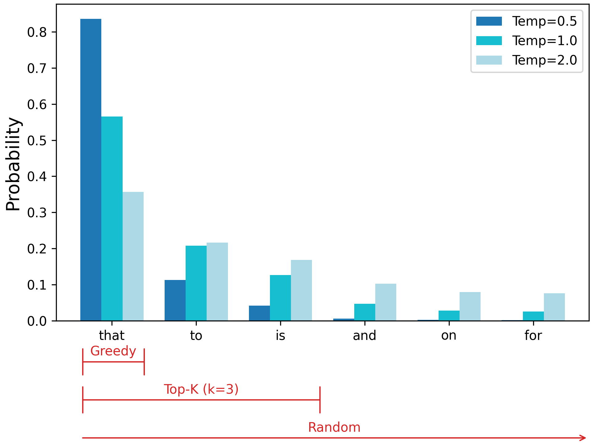
Another popular technique for shaping our distribution is restricting our sampling to a set of the most likely tokens. This is called top-K sampling, where K is the number of candidates you should explore. Figure 16.3 shows how top-K sampling strikes a middle ground between greedy and random approaches.
Let’s try this out in code. We can use op_top_k() to find the top K elements of an array:
top_k <- function(preds, k = 5, temperature = 1) {
  preds <-  preds / temperature
  .[top_preds, top_indices] <- op_top_k(preds, k = k, sorted = FALSE)
  choice <- random_sample(top_preds)
  op_take(top_indices, choice)
}
We can try a few different variations of top-K to see how it affects sampling:
compiled_generate(prompt, \(preds) top_k(preds, k = 5))A piece of advice that I can't help it. I'm not going to be able to do anything
for a few months, but I'm trying to get a little better. It's a little too much.
I have a few other questions on this site, but I'm sure Icompiled_generate(prompt, \(preds) top_k(preds, k = 20))A piece of advice and guidance from the Audi Bank in 2015. With all the above,
it’s not just a bad idea, but it’s very good to see that is going to be a great
year for you in 2017.
That’s really going toPassing a top-K cutoff is different than temperature sampling. Passing a low temperature makes likely tokens more likely, but it does not rule out any token. Top-K sampling zeros out the probability of anything outside the K candidates. We can combine the two—for example, sampling the top five candidates with a temperature of 0.5:
compiled_generate(prompt, \(preds) top_k(preds, k = 5, temperature=0.5))A piece of advice that you can use to get rid of the problem.
The first thing you need to do is to get the job done. It is important that you
have a plan that will help you get rid of it.
The first thing you need to do is to get rid of the problem yourself.A sampling strategy is an important control when generating text, and there are many more approaches. For example, beam search is a technique that heuristically explores multiple chains of predicted tokens by keeping a fixed number of “beams” (different chains of predicted tokens) to explore at each timestep.
With top-K sampling, our model generates something closer to plausible English text, but there is little apparent utility to such output. This fits with the results of GPT-1. For the initial GPT paper, the generated output was more of a curiosity, and state-of-the-art results were achieved only by fine-tuning classification models. Our mini-GPT is far less trained than GPT-1.
To reach the scale of generative LLMs today, we’d need to increase our parameter count by at least 100 times and our train step count by at least 1,000 times. If we did, we would see the same leaps in quality observed by OpenAI with GPT. And we could do it! The training recipe we used previously is the exact blueprint used by everyone training LLMs today. The only missing pieces are a very large compute budget and some tricks for training across multiple machines that we will cover in chapter 18.
For a more practical approach, we will transition to using a pretrained model. This will allow us to explore the behavior of an LLM at today’s scale.
16.3 Using a pretrained LLM
Now that we’ve trained a mini-language model from scratch, let’s try using a billion-parameter pretrained model and see what it can do. Given how prohibitively expensive pretraining a Transformer can be, most of the industry has centered around using pretrained models developed by a relatively short list of companies. This is not purely a cost concern but also an environmental one: generative model training is now making up a large fraction of the total data center power consumption of large tech companies.
Meta issued some environmental data on Llama 2, an LLM it published in 2023. It’s a good bit smaller than GPT-3, but it needed an estimated 1.3 million kilowatt hours of electricity to train—the daily power usage of about 45,000 American households. If every organization using an LLM ran pretraining itself, the scale of energy use would be a noticeable fraction of global energy consumption.
Let’s play around with a pretrained generative model from Google called Gemma. We will use the third version of the Gemma model, which was released to the public in 2025. To keep the examples in this book accessible, we will use the smallest variation of Gemma available, which clocks in at almost exactly 1 billion parameters. This “small” model was trained on roughly 2 trillion tokens of pretraining data—2,000 times more tokens than the mini-GPT we just trained!
16.3.1 Text generation with the Gemma model
To load this pretrained model, we can use KerasHub as we have done in previous chapters.
NoteAccessing Gemma’s weights
If you are running the code for this chapter yourself, you will need to accept the terms of use for the Gemma models before you can download the weights. The model weights are stored on Kaggle, and you can use the kagglehub API to log in as in chapter 8. Before you do, you will need to do two things:
- Go to https://www.kaggle.com/models/keras/gemma3 and accept the Gemma terms of use at the top of the page.
- Go to https://www.kaggle.com/settings and generate a Kaggle API Key (if you did not already do this in chapter 8; see chapter 8 for more detailed instructions).
If you are running this in Colab, you can instead authenticate via the browser, like this:
py_require("kagglehub")
import("kagglehub")$login()
As LLMs become increasingly powerful, terms of service like this are becoming more common. The Gemma terms of use prohibit using the model for things like generating spam or hate speech.
py_require("keras-hub")
keras_hub <- import("keras_hub")

gemma_lm <- keras_hub$models$CausalLM$from_preset(
  "gemma3_1b",
  dtype = "float32"
)
CausalLM is another example of the high-level task API, much like the ImageClassifier and ImageSegmenter tasks we used earlier in the book. The CausalLM task will combine a tokenizer and correctly initialized architecture into a single Keras model. KerasHub will load the Gemma weights into a correctly initialized architecture and load a matching tokenizer for the pretrained weights.
Let’s take a look at the Gemma model summary:
gemma_lmPreprocessor: "gemma3_causal_lm_preprocessor"
┏━━━━━━━━━━━━━━━━━━━━━━━━━━━━━━━━━━━━━━━━━━━━┳━━━━━━━━━━━━━━━━━━━━━━━━━━━━━┓
┃ Layer (type) ┃ Config ┃
┡━━━━━━━━━━━━━━━━━━━━━━━━━━━━━━━━━━━━━━━━━━━━╇━━━━━━━━━━━━━━━━━━━━━━━━━━━━━┩
│ gemma3_tokenizer (Gemma3Tokenizer) │ Vocab size: 262,144 │
└────────────────────────────────────────────┴─────────────────────────────┘
Model: "gemma3_causal_lm"
┏━━━━━━━━━━━━━━━━━━━━━┳━━━━━━━━━━━━━━━━━━━┳━━━━━━━━━━━━┳━━━━━━━━━━━━━━━━━━━┓
┃ Layer (type) ┃ Output Shape ┃ Param # ┃ Connected to ┃
┡━━━━━━━━━━━━━━━━━━━━━╇━━━━━━━━━━━━━━━━━━━╇━━━━━━━━━━━━╇━━━━━━━━━━━━━━━━━━━┩
│ padding_mask │ (None, None) │ 0 │ - │
│ (InputLayer) │ │ │ │
├─────────────────────┼───────────────────┼────────────┼───────────────────┤
│ token_ids │ (None, None) │ 0 │ - │
│ (InputLayer) │ │ │ │
├─────────────────────┼───────────────────┼────────────┼───────────────────┤
│ gemma3_backbone │ (None, None, │ 999,885,9… │ padding_mask[0][… │
│ (Gemma3Backbone) │ 1152) │ │ token_ids[0][0] │
├─────────────────────┼───────────────────┼────────────┼───────────────────┤
│ token_embedding │ (None, None, │ 301,989,8… │ gemma3_backbone[… │
│ (ReversibleEmbeddi… │ 262144) │ │ │
└─────────────────────┴───────────────────┴────────────┴───────────────────┘
Total params: 999,885,952 (3.72 GB)
Trainable params: 999,885,952 (3.72 GB)
Non-trainable params: 0 (0.00 B)
Rather than implementing a generation routine ourselves, we can simplify our lives by using the generate() function that comes as part of the CausalLM class. This function can be compiled with different sampling strategies, as we explored in the previous section:
gemma_lm$compile(sampler = "greedy")
cat(gemma_lm$generate("A piece of advice", max_length = 40L))
A piece of advice from a former student of mine:
<blockquote>“I’m not sure if you’ve heard of it, but I’ve been told
that the best way to learncat(gemma_lm$generate("How can I make brownies?", max_length = 40L))How can I make brownies?
[User 0001]
I'm trying to make brownies for my son's birthday party. I've never
made brownies before.You’ll notice a few things right off the bat. First, the output is much more coherent than our mini-GPT model. It would be hard to distinguish this text from much of the training data in the C4 dataset. Second, the output is still not that useful. The model generates vaguely plausible text, but what you could do with it is unclear.
As with the mini-GPT example, this is not so much a bug as a consequence of our pretraining objective. The Gemma model was trained with the same “guess the next word” objective we used for mini-GPT, which means it’s effectively a fancy autocomplete for the internet. It will just keep rattling off the most probable word in its single sequence as if our prompt was a snippet of text found in a random document on the web.
One way to change our output is to prompt the model with a longer input that makes it obvious the type of output we are looking for. For example, if we prompt the Gemma model with the beginning two sentences of a brownie recipe, we get more helpful output:
gemma_lm$generate(
  paste0(
    "The following brownie recipe is easy to make in just a few steps.",
    "\n\nYou can start by"
  ),
  max_length = 40L
) |> cat()
The following brownie recipe is easy to make in just a few steps.
You can start by melting the butter and sugar in a saucepan over
medium heat.
Then add the eggs and vanilla extractAlthough it’s tempting when working with a model that can “talk” to imagine it interpreting our prompt in some sort of human, conversational way, nothing of the sort is going on here. We have just constructed a prompt for which an actual brownie recipe is a more likely continuation than mimicking someone posting on a forum asking for baking help.
You can go much further in constructing prompts. You might prompt a model with some natural language instructions of the role it is supposed to fill, for example “You are a large language model that gives short, helpful answers to people’s questions.” Or you might feed the model a prompt containing a long list of harmful topics that should not be included in any generated responses.
If this all sounds a bit hand-wavy and hard to control, that’s a good assessment. Attempting to visit different parts of a model’s distribution through prompting is often useful, but predicting how a model will respond to a given prompt is very difficult.
Another well-documented problem faced by LLMs is “hallucinations.” A model will always say something—there is always a most likely next token to a given sequence. Finding locations in our LLM distribution that have no grounding in actual fact is easy:
gemma_lm$generate(
  "Tell me about the 542nd president of the United States.",
  max_length = 40L
) |> cat()
Tell me about the 542nd president of the United States.
The 542nd president of the United States was James A. Garfield.Of course, this is utter nonsense, but the model could not find a more likely way to complete this prompt.
Hallucinations and uncontrollable output are fundamental problems with language models. If there is a silver bullet, we have yet to find it. However, one approach that helps immensely is to further fine-tune a model with examples of the specific types of generative outputs you would like.
In the specific case of wanting to build a chatbot that can follow instructions, this type of training is called instruction fine-tuning. Let’s try some instruction fine-tuning with Gemma to make it a lot more useful as a conversation partner.
16.3.2 Instruction fine-tuning
Instruction fine-tuning involves feeding the model input/output pairs: a user instruction followed by a model response. We combine these into a single sequence that becomes new training data for the model. To make it clear during training when an instruction or response ends, we can add special markers like "[instruction]" and "[response]" directly to the combined sequence. The precise markup will not matter much, as long as it is consistent.
We can use the combined sequence as regular training data, with the same “guess the next word” loss we used to pretrain an LLM. By doing further training with examples containing desired responses, we are essentially bending the model’s output in the direction we want. We won’t be learning a latent space for language here; that’s already been done over trillions of tokens of pretraining. We are simply nudging the learned representation a bit to control the tone and content of the output.
To begin, we will need a dataset of instruction–response pairs. Training chatbots is a hot topic, so there are many datasets made specifically for this purpose. We will use a dataset made public by the company Databricks. Employees contributed to a dataset of 15,000 instructions and handwritten responses. Let’s download it and join the data into a single sequence.
library(dplyr, warn.conflicts = FALSE)

format_prompt <-
  \(instruction) paste0("[instruction]\n", instruction, "[end]\n[response]\n")
format_response <-
  \(response) paste0(response, "[end]")


dataset_path <- get_file(origin = paste0(
  "https://hf.co/datasets/databricks/databricks-dolly-15k/",
  "resolve/main/databricks-dolly-15k.jsonl"
))

data <- readr::read_lines(dataset_path) |>
  lapply(jsonlite::parse_json) |>
  bind_rows()

glimpse(data)
Rows: 15,011
Columns: 4
$ instruction <chr> "When did Virgin Australia start operating?", "Which i…
$ context <chr> "Virgin Australia, the trading name of Virgin Australi…
$ response <chr> "Virgin Australia commenced services on 31 August 2000…
$ category <chr> "closed_qa", "classification", "open_qa", "open_qa", "…
data <- data |>
  filter(context == "") |>
  mutate(
    prompts = format_prompt(instruction),
    responses = format_response(response),
    .keep = 'none'
  )
Note that some examples have additional context—textual information related to the instruction. To keep things simple for now, we will discard those examples.
Let’s take a look at a single element in our dataset:
str(data[2,])tibble [1 × 2] (S3: tbl_df/tbl/data.frame)
$ prompts : chr "[instruction]\nWhy can camels survive for long without water?[end]\n[response]\n"
$ responses: chr "Camels use the fat in their humps to keep them filled with energy and hydration for long periods of time.[end]"Our prompt template gives our examples a predictable structure. Although Gemma is not a sequence-to-sequence model like our English-to-Spanish translator, we can still use it in a sequence-to-sequence setting by training on prompts like this and generating the output only after the "[response]" marker.
Let’s make a tf.data.Dataset and split some validation data:
library(tfdatasets, exclude = "shape")

ds <- data |>
  tensor_slices_dataset() |>
  dataset_shuffle(2000) |>
  dataset_batch(2)

val_ds <- ds |> dataset_take(100)
train_ds <- ds |> dataset_skip(100)
The CausalLM we loaded from the KerasHub library is a high-level object for end-to-end causal language modeling. It wraps two objects: a preprocessor layer, which preprocesses text input, and a backbone model, which contains the numerics of the model forward pass. Preprocessing is included by default in high-level Keras functions like fit() and predict(). But let’s run our preprocessing on a single batch so we can better see what it is doing:
preprocessor <- gemma_lm$preprocessor
preprocessor$sequence_length <- 512L
batch <- iter_next(as_iterator(train_ds))
.[x, y, sample_weight] <- preprocessor(batch)
str(x)
List of 2
$ token_ids : <jax.Array shape(2, 512), dtype=int32>
$ padding_mask: <jax.Array shape(2, 512), dtype=bool>str(y)<jax.Array shape(2, 512), dtype=int32>str(sample_weight)<jax.Array shape(2, 512), dtype=bool>The preprocessor layer pads all inputs to a fixed length and computes a padding mask to track which token ID inputs are just padded zeros. The sample_weight tensor allows us to compute a loss value only for our response tokens. We don’t really care about the loss for the user prompt, because it is fixed, and we definitely don’t want to compute the loss for the zero padding we just added.
If we print a snippet of our token IDs and labels, we can see that this is just the regular language model setup, where each label is the next token value:
# bind
rbind(x$token_ids |> as.array() |> _[1, 1:5],
      y |> as.array() |> _[1, 1:5])
[,1] [,2] [,3] [,4] [,5]
[1,] 2 236840 22768 236842 107
[2,] 236840 22768 236842 107 598616.3.3 Low-Rank Adaptation (LoRA)
If we ran fit() right now on a Colab GPU with 16 GB of device memory, we would quickly trigger an out-of-memory error. But we’ve already loaded the model and run generation, so why would we run out of memory now?
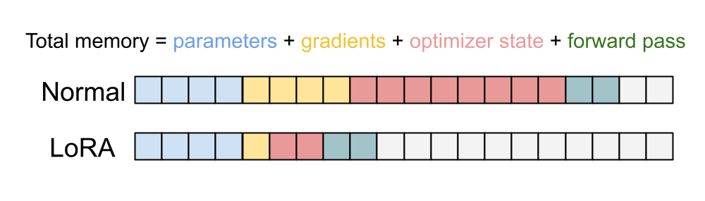
Our 1-billion-parameter model takes up about 3.7 GB of memory; you can see it in our previous model summary. The Adam optimizer we have been using will need to track three extra floating-point numbers for each parameter: the actual gradients, a velocity value, and a momentum value. All told, it comes out to 15 GB just for the weights and optimizer state. We also need a few gigabytes of memory to keep track of intermediate values in the forward pass of the model, but we have none left to spare. Running fit() would crash on the first train step. This is a common problem when training LLMs. Because these models have large parameter counts, the throughput of our GPUs and CPUs is a secondary concern to fitting the model on accelerator memory.
You saw earlier in this book how to freeze certain parts of a model during fine-tuning. What we did not mention is that this saves a lot of memory! We do not need to track any optimizer variables for frozen parameters—they will never update. This allows us to save considerable space on an accelerator.
Researchers have experimented extensively with freezing different parameters in a Transformer model during fine-tuning, and it turns out, perhaps intuitively, that the most important weights to leave unfrozen are in the attention mechanism. But our attention layers still have hundreds of millions of parameters. Can we do even better?
In 2021, researchers at Microsoft proposed a technique called Low-Rank Adaptation of Large Language Models (LoRA) specifically to solve this memory problem.3 To explain it, let’s imagine a simple linear projection layer:
layer_linear <- new_layer_class(
  classname = "Linear",
  initialize = function(input_dim, output_dim) {
    super$initialize()
    self$kernel <- self$add_weight(shape = shape(input_dim, output_dim))
  },
  call = function(inputs) {
1    inputs %*% self$kernel
  }
)- 1
-
%*%callsop_matmul()
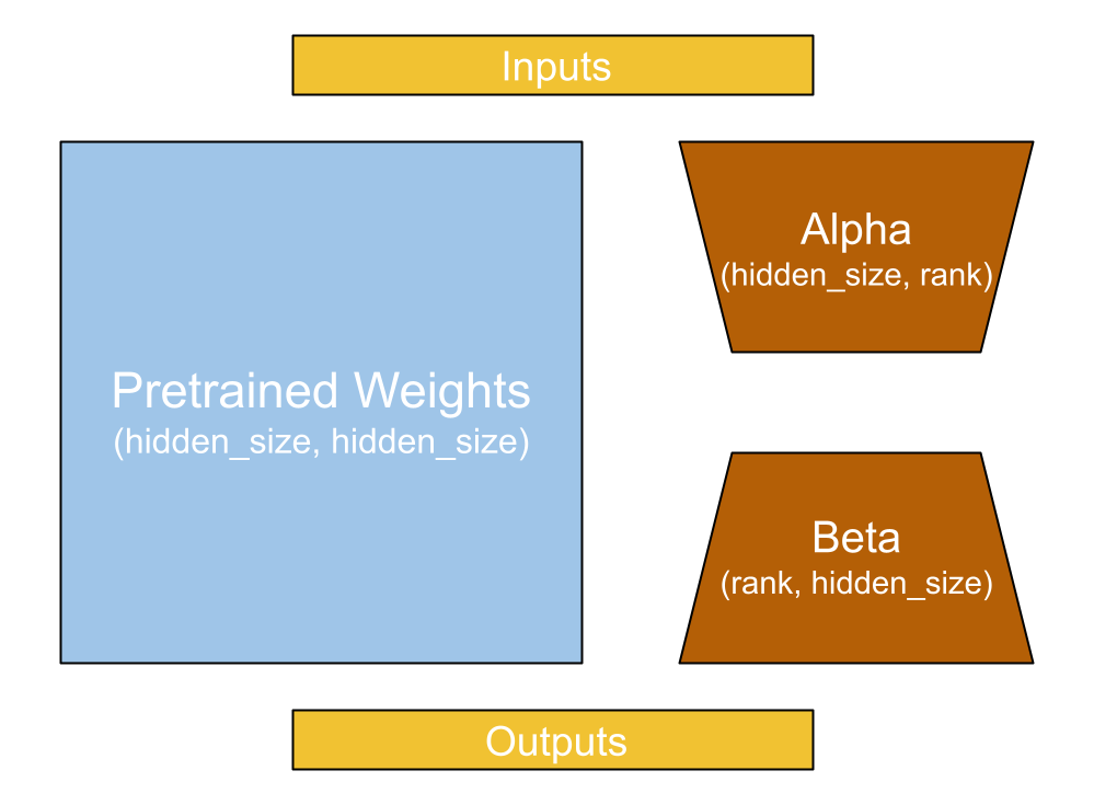
The LoRA paper proposes freezing the kernel matrix and adding a new “low rank” decomposition of the kernel projection. This decomposition has two new projection matrices, alpha and beta, which project to and from an inner rank. Let’s take a look:
layer_lora_linear <- new_layer_class(
  classname = "LoraLinear",
  initialize = function(input_dim, output_dim, rank) {
    super$initialize()
    self$kernel <- self$add_weight(shape(input_dim, output_dim),
                                   trainable = FALSE)
    self$alpha <- self$add_weight(shape(input_dim, rank))
    self$beta <- self$add_weight(shape(rank, output_dim))
  },
  call = function(inputs) {
    frozen <- inputs %*% self$kernel
    update <- inputs %*% self$alpha %*% self$beta
    frozen + update
  }
)
If our kernel is shape 2,048 × 2,048, that is 4,194,304 frozen parameters. But if we keep the rank low, say 8, we would have only 32,768 parameters for the low-rank decomposition. This update will not have the same expressive power as the original kernel; at the narrow middle point, the entire update must be represented as eight floats. But during LLM fine-tuning, we no longer need the expressive power required during pretraining (figure 16.4).
The LoRA authors suggest freezing the entire Transformer and adding LoRA weights only to the query and key projections in the attention layer. Let’s try that. KerasHub models have a built-in method for LoRA training.
gemma_lm$backbone$enable_lora(rank = 8L)
NoteCustomizing LoRA training
The enable_lora() method is also available on individual Dense layers. We could equivalently write the previous call, a little more verbosely, by iterating through the layers of the Transformer:
1gemma_lm$backbone$trainable <- FALSE
for (i in seq_len(gemma_lm$backbone$num_layers) - 1) {
2  layer <- get_layer(gemma_lm$backbone, sprintf("decoder_block_%d", i))
  layer$attention$key_dense$trainable <- TRUE
  layer$attention$key_dense$enable_lora(rank = 8L)
  layer$attention$query_dense$trainable <- TRUE
  layer$attention$query_dense$enable_lora(rank = 8L)
}- 1
- Set all layers to not be trainable.
- 2
- Make key and query projections trainable and enable LoRA.
With this approach, we could add more trainable parameters earlier or later in the model, or also add LoRA to the value projection.
Let’s look at our model summary again:
gemma_lmPreprocessor: "gemma3_causal_lm_preprocessor"
┏━━━━━━━━━━━━━━━━━━━━━━━━━━━━━━━━━━━━━━━━━━━━┳━━━━━━━━━━━━━━━━━━━━━━━━━━━━━┓
┃ Layer (type) ┃ Config ┃
┡━━━━━━━━━━━━━━━━━━━━━━━━━━━━━━━━━━━━━━━━━━━━╇━━━━━━━━━━━━━━━━━━━━━━━━━━━━━┩
│ gemma3_tokenizer (Gemma3Tokenizer) │ Vocab size: 262,144 │
└────────────────────────────────────────────┴─────────────────────────────┘
Model: "gemma3_causal_lm"
┏━━━━━━━━━━━━━━━━━━━┳━━━━━━━━━━━━━━━━━┳━━━━━━━━━━━┳━━━━━━━━━━━━━━━━┳━━━━━━━┓
┃ Layer (type) ┃ Output Shape ┃ Param # ┃ Connected to ┃ Trai… ┃
┡━━━━━━━━━━━━━━━━━━━╇━━━━━━━━━━━━━━━━━╇━━━━━━━━━━━╇━━━━━━━━━━━━━━━━╇━━━━━━━┩
│ padding_mask │ (None, None) │ 0 │ - │ - │
│ (InputLayer) │ │ │ │ │
├───────────────────┼─────────────────┼───────────┼────────────────┼───────┤
│ token_ids │ (None, None) │ 0 │ - │ - │
│ (InputLayer) │ │ │ │ │
├───────────────────┼─────────────────┼───────────┼────────────────┼───────┤
│ gemma3_backbone │ (None, None, │ 1,001,19… │ padding_mask[… │ Y │
│ (Gemma3Backbone) │ 1152) │ │ token_ids[0][… │ │
├───────────────────┼─────────────────┼───────────┼────────────────┼───────┤
│ token_embedding │ (None, None, │ 301,989,… │ gemma3_backbo… │ N │
│ (ReversibleEmbed… │ 262144) │ │ │ │
└───────────────────┴─────────────────┴───────────┴────────────────┴───────┘
Total params: 1,001,190,528 (3.73 GB)
Trainable params: 1,304,576 (4.98 MB)
Non-trainable params: 999,885,952 (3.72 GB)
Although our model parameters still occupy 3.7 GB of space, our trainable parameters now use only 5 MB of data—a thousandfold decrease! This can take our optimizer state from many gigabytes to just megabytes on the GPU (figure 16.5).
With this optimization in place, we are at last ready to instruction-tune our Gemma model. Let’s give it a go.
gemma_lm |> compile(
  loss = loss_sparse_categorical_crossentropy(from_logits = TRUE),
  optimizer = optimizer_adam(5e-5),
  weighted_metrics = metric_sparse_categorical_accuracy()
)
gemma_lm |> fit(train_ds, validation_data = val_ds, epochs = 1)
After training, we get to 55% accuracy when guessing the next word in our model’s response. That’s a huge jump from the 35% accuracy of our mini-GPT model. This shows the power of a larger model and more extensive pretraining.
Did our fine-tuning make our model better at following directions? Let’s give it a try:
gemma_lm$generate(
  format_prompt("How can I make brownies?"),
  max_length = 512L
)
[instruction]
How can I make brownies?[end]
[response]
You can make brownies by mixing together 1 cup of flour, 1 cup of sugar, 1/2
cup of butter, 1/2 cup of milk, 1/2 cup of chocolate chips, and 1/2 cup of
chocolate chips. Then, you can bake it in a 9x13 pan for 30 minutes at 350
degrees Fahrenheit. You can also add a little bit of vanilla extract to the
batter to make it taste better.[end]gemma_lm$generate(
format_prompt("What is a proper noun?"),
max_length = 512L
) |> cat()[instruction]
What is a proper noun?[end]
[response]
A proper noun is a word that refers to a specific person, place, or thing.
Proper nouns are usually capitalized and are used to identify specific
individuals, places, or things. Proper nouns are often used in formal writing
and are often used in titles, such as "The White House" or "The Eiffel Tower."
Proper nouns are also used in titles of books, movies, and other works of
literature.[end]Much better. Our model will now respond to questions, instead of trying to simply carry on the thought of the prompt text.
Have we solved the hallucination problem?
gemma_lm$generate(
  format_prompt("Who is the 542nd president of the United States?"),
  max_length = 512L
) |> cat()
[instruction]
Who is the 542nd president of the United States?[end]
[response]
The 542nd president of the United States was James A. Garfield.[end]Not at all. However, we could still use instruction tuning to make some inroads here. A common technique is to train the model on a lot of instruction/response pairs where the desired response is “I don’t know” or “As a language model, I cannot help you with that.” This can train the model to avoid attempting to answer specific topics where it would often give poor-quality results.
16.4 Going further with LLMs
We have now trained a GPT model from scratch and fine-tuned a language model into our very own chatbot. However, we are just scratching the surface of LLM research today. In this section, we will cover a nonexhaustive list of extensions and improvements to the basic “autocomplete the internet” language modeling setup.
16.4.1 Reinforcement learning with human feedback (RLHF)
The type of instruction fine-tuning we just did is often called supervised fine-tuning. It is supervised because we are curating, by hand, a list of example prompts and responses we want from the model.
Any need to manually write text examples will almost always become a bottleneck; such data is slow and expensive to come by. Moreover, this approach will be limited by the human performance ceiling on the instruction-following task. If we want to do better than human performance in a chatbot-like experience, we cannot rely on manually written output to supervise LLM training.
The real problem we are trying to optimize is our preference for certain responses over others. With a large enough sample of people, this preference problem is perfectly defined, but figuring out how to translate from “our preferences” to a loss function we could use to compute gradients is tricky. This is what reinforcement learning with human feedback (RLHF) attempts to solve. OpenAI originally described RLHF in a 2022 paper4 and used this training setup to go from GPT-3’s initial, pretrained parameters to the first version of ChatGPT.
The first step in RLHF fine-tuning is exactly what we did in the last section: supervised fine-tuning with handwritten prompts and responses. This gets us to a good baseline performance; we now need to improve on this baseline. To this aim, we will build a reward model that can act as a proxy for human preference. We can gather a large number of prompts and responses to these prompts. Some of these responses can be handwritten; the model can write others. Responses could even be written by other chatbot LLMs. We then need to get human evaluators to rank these responses by preference. Given a prompt and several potential responses, an evaluator’s task is to rank them from most helpful to least helpful. Such data collection is expensive and slow but still faster than writing all the desired responses by hand.
We can use this ranked-preference dataset to build the reward model, which takes in a prompt–response pair and outputs a single floating-point value. The higher the value, the better the response. This reward model is usually another, smaller Transformer. Instead of predicting the next token, it reads a whole sequence and outputs a single float: a rating for a given response.
We can then use this reward model to tune our model further, using a reinforcement learning setup. We won’t get too deep into the details of reinforcement learning in this book, but don’t be intimidated by the term—it refers to any training setup where a deep learning model learns by making predictions (called actions) and getting feedback on that output (called rewards). In short, a model’s own predictions become its training data.
In our case, the action is simply generating a response to an input prompt, as we have been doing with the generate() function. The reward is simply applying a separate regression model to that string output. Here’s a simple example in pseudocode.
- 1
- Take an action.
- 2
- Receive a reward.
- 3
- Update the model parameters. We do not update the reward model.
In this example, we filter our generated responses with a reward cutoff and treat the “good” output as new training data for more supervised fine-tuning, as we did in the last section. In practice, you usually won’t discard bad responses but rather will use specialized gradient update algorithms to steer your model’s parameters using all responses and rewards. After all, a bad response gives a good signal for what not to do.
An advantage of this setup is that it can be iterative. We can take this newly trained model, generate new and improved responses to prompts, rank these responses by human preference, and train a new and improved reward model.
16.4.1.1 Using a chatbot trained with RLHF
We can make this more concrete by trying a model trained with this form of iterative preference tuning. Because building chatbots is the “killer app” for large Transformer models, it is common practice for companies that release pretrained models like Gemma to release specialized “instruction-tuned” versions, built just for chat. Let’s try loading one now. This will be a 4-billion-parameter model, quadruple the size of the model we just loaded and the largest model we will use in this book.
gemma_lm <- keras_hub$models$CausalLM$from_preset(
  "gemma3_instruct_4b",
  dtype = "float16"
)
NoteChoosing a dtype for large models
You might have noticed we passed dtype = "float32" when creating our Gemma model the first time, and dtype = "float16" now. What is going on?
For models like Gemma with more than a billion parameters, the number of bytes used for each floating-point number is an important consideration. When you are training a model, it is often a good idea to use 32 bits (4 bytes) per parameter. Thirty-two-bit floats can represent very small values, which can help keep training gradients stable. Here we aren’t doing any training, so we pass float16, which uses only 2 bytes per parameter. We don’t need to worry about gradient stability, and we will save many gigabytes of memory by using a lower precision. If you have a newer GPU, you can also try passing "bfloat16".
There’s a detailed discussion of floating-point precision, and of the difference between "float16" and "bfloat16", coming up in chapter 18.
Like the earlier Gemma model we fine-tuned ourselves, this instruction-tuned checkpoint comes with a specific template for formatting its input. Again, the exact text does not matter; what is important is that our prompt template matches what was used to tune the model:
template_format <- \(prompt) paste0(
  "<start_of_turn>user\n", prompt,
  "<end_of_turn>\n<start_of_turn>model"
)
Let’s try asking it a question:
prompt <- "Why can't you assign values in Jax tensors? Be brief!"
cat(gemma_lm$generate(template_format(prompt), max_length = 512L))
<start_of_turn>user
Why can't you assign values in Jax tensors? Be brief!<end_of_turn>
<start_of_turn>model
Jax tensors are designed for efficient automatic differentiation. Directly
assigning values disrupts this process, making it difficult to track gradients
correctly. Instead, Jax uses operations to modify tensor values, preserving the
differentiation pipeline.<end_of_turn>This 4-billion-parameter model was first pretrained on 14 trillion tokens of text and then extensively fine-tuned to make it more helpful when answering questions. Some of this tuning was done with supervised fine-tuning as we did in the previous section, some with RLHF as we covered in this section, and some with still other techniques—like using an even larger model as a “teacher” to guide training. The increase in ability to answer questions is easily noticeable.
Let’s try this model on the prompt that has been giving us trouble with hallucinations:
prompt <- "Who is the 542nd president of the United States?"
cat(gemma_lm$generate(template_format(prompt), max_length = 512L))
<start_of_turn>user
Who is the 542nd president of the United States?<end_of_turn>
<start_of_turn>model
This is a trick question! As of today, November 2, 2023, the United States has
only had 46 presidents. There hasn't been a 542nd president yet. 😊
You're playing with a very large number!<end_of_turn>This more capable model refuses to take the bait. This is not the result of a new modeling technique, but rather the result of extensive training on trick questions like this one, with responses like the one we just received. In fact, you can see clearly here why removing hallucinations can be a bit like playing whack-a-mole—even though it refused to hallucinate a US president, the model now manages to make up today’s date.
16.4.2 Multimodal LLMs
One obvious chatbot extension is the ability to handle new modalities of input. An assistant that can respond to audio input and process images would be far more useful than one that can only operate on text.
Extending a Transformer to different modalities can be done in a conceptually simple way. The Transformer is not a text-specific model; it’s a highly effective model for learning patterns in sequence data. If we can figure out how to coerce other data types into a sequence representation, we can feed this sequence into a Transformer and train with it.
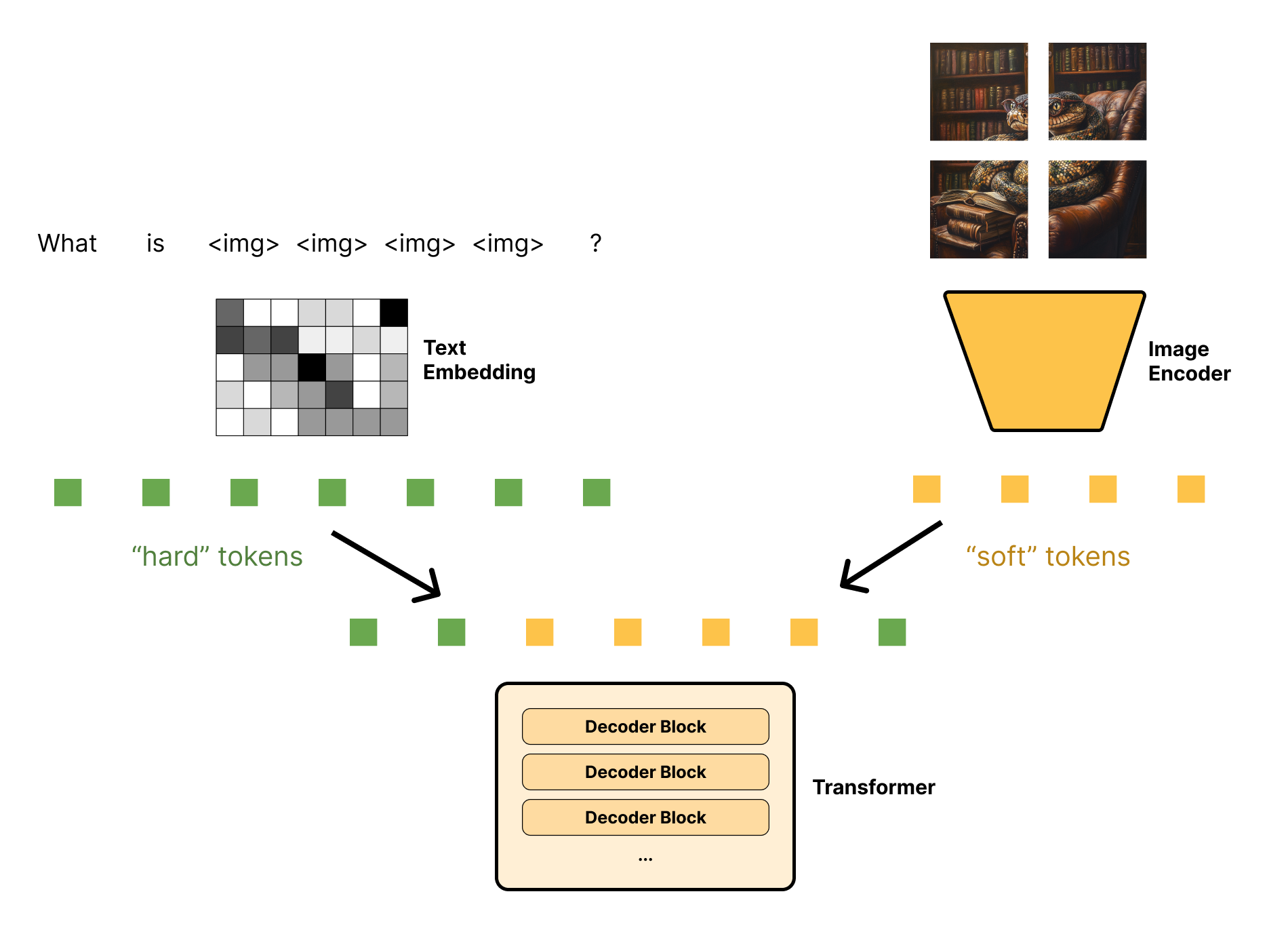
In fact, the Gemma model we just loaded does just that. The model comes with a separate, 420-million-parameter image encoder that cuts an input image into 256 patches and encodes each patch as a vector with the same dimensionality as Gemma’s hidden Transformer dimension. Each image will be embedded as a (256, 2560) sequence. Because 2560 is the hidden dimensionality of the Gemma Transformer model, this image representation can simply be spliced into our text sequence after the token embedding layer. You can think of it like 256 special tokens representing the image, where each (1, 2560) vector is sometimes called a soft token (figure 16.6). Unlike our normal hard tokens, where each token ID can only take on a fixed number of possible vectors in our token embedding matrix, these image soft tokens can take on any vector value output by the vision encoder.
Let’s load an image to see how this works in a little more detail (see figure 16.7):
image_url <- paste0("https://github.com/mattdangerw/keras-nlp-scripts/",
                    "blob/main/learned-python.png?raw=true")
image_path <- get_file(origin = image_url)

image <- image_path |> image_load() |> image_to_array()
par(mar = c(0, 0, 0, 0))
plot(as.raster(image, max = 255L))
We can use Gemma to ask some questions about this image:
1gemma_lm$preprocessor$max_images_per_prompt <- 1L
gemma_lm$preprocessor$sequence_length <- 512L
prompt <- "What is going on in this image? Be concise!<start_of_image>"
gemma_lm$generate(list(
  prompts = template_format(prompt),
  images = list(image)
))- 1
- Limits the maximum input size of the model
<start_of_turn>user
What is going on in this image? Be concise!

<start_of_image>

<end_of_turn>
<start_of_turn>model
A snake wearing glasses is sitting in a leather armchair, surrounded by a large
bookshelf, and reading a book. It’s a whimsical, slightly surreal image.
<end_of_turn>
prompt = "What is the snake wearing?<start_of_image>"
gemma_lm$generate(list(
prompts = template_format(prompt),
images = list(image)
))<start_of_turn>user
What is the snake wearing?
<start_of_image>
<end_of_turn>
<start_of_turn>model
The snake is wearing a pair of glasses! They are red-framed and perched on its
head.<end_of_turn>Each of our input prompts contains the special token <start_of_image>. This is turned into 256 placeholder values in our input sequence, which, in turn, are replaced with the soft tokens representing our image.
Training for a multimodal model like this is similar to regular LLM pretraining and fine-tuning. Usually, we would first pretrain our image encoder separately, as we first did in chapter 8 of this book. Then we can do the same basic “guess the next word” pretraining and also feed in mixed image and text content combined into a single sequence. Our Transformer would not be trained to output image soft tokens; we would simply zero the loss at these image-token locations.
It might seem almost magical that we can add image data to an LLM, but when we consider the power of the sequence model we’re working with, it’s really an expected result. We’ve taken a Transformer, recast our image input as sequence data, and done a lot of extra training. The model can preserve the original language model’s ability to ingest and produce text while learning to also embed images in the Transformer’s latent space.
16.4.2.1 Foundation models
As LLMs venture into different modalities, the “large language model” moniker can become a bit misleading. They do model language, but also images, audio, and maybe even structured data. In the next chapter, you will see a distinct architecture, called diffusion models: they work differently in terms of underlying structure but have a similar feel—they too are trained on massive amounts of data at “internet scale” with a self-supervised loss.
An umbrella term for models like this is foundation models. More specifically, a foundation model is any model that is trained on broad data (generally using self-supervision at scale) that can be fine-tuned to a wide range of downstream tasks.
In general, you can think of a foundation model as learning to reconstruct data pulled from large swaths of the internet, given a partial representation of it. Although LLMs are the first and best known of these models, there are many others. The hallmarks of a foundation model are the self-supervised learning objective (a reconstruction loss) and the fact that these models are not specialized to a single task and can be used for a number of downstream purposes.
This is an important, and striking, shift that has happened quite recently in the long history of machine learning. Rather than training a model from scratch on your individual dataset, you will often be better off using a foundation model to get a rich representation of your input (whether it’s images, text, or something else) and then specializing that model for your final downstream task. Of course, this comes with the downside of needing to run large models with billions of parameters, so it’s hardly a fit for all real-world applications of machine learning.
16.4.3 Retrieval-augmented generation (RAG)
Sticking extra information in the prompt is not helpful only in handling image data; it can be a general way to extend the capabilities of an LLM. One notable example is when using an LLM for search. If we naively compare an LLM to a search engine, it has a couple of fatal flaws:
- As we’ve mentioned previously, an LLM will occasionally make things up. It will output false “facts” that were not present in the training data but could be interpolated from the training data. This information can range from misleading to dangerous.
- An LLM’s knowledge of the world has a cutoff date—at best, the date the model was pretrained. Training an LLM is expensive, and it is not feasible to train continuously on new data. So, at some arbitrary point in time, an LLM’s knowledge of the world stops.
No one wants to use a search engine that can only tell you about things that happened six months ago. But if we think of an LLM as more like “conversational software” that can handle any sequence data in a prompt, what if we instead used the model as the interface to information retrieved by more traditional search? That’s the idea behind retrieval-augmented generation (RAG).
RAG works by taking an initial user question and doing a query to pull in additional text context. This query can be sent to a database, a search engine, or anything that can give further information on the question asked by a user. This extra information is then added straight into the prompt. For example, we might construct a prompt like this:
Use the following pieces of context to answer the question.
Question: What are some good ways to improve sleep?
Context: {text from a medical journal on improving sleep}
Answer:
A common approach for looking up relevant information is to use a vector database. To build a vector database, we can use an LLM or any model to embed a series of source documents as vectors. The document text is stored in the database, with the embedding vector used as a key. During retrieval, an LLM can again be used to embed the user query as a vector. The vector database is responsible for searching for key vectors close to the query vector and for surfacing the corresponding text. This might sound a lot like the attention mechanism itself—recall that the terms query, key, and value came from database systems.
Surfacing information to assist with generation does a few things:
- It gives us an obvious way to work around the cutoff date of the model.
- It allows the model to access private data. Companies might want to use an LLM trained on public data to serve as an interface to information stored privately.
- It can help factually ground the model. There is no silver bullet that stops hallucinations entirely, but an LLM is much less likely to make up facts on a topic if presented with correct context about the subject in a prompt.
Tip
You can use ragnar (https://ragnar.tidyverse.org) to implement RAG workflows. It provides transparent, configurable tools for every step: reading, chunking, and embedding documents; building a vector store; and retrieving text with support for hybrid vector and BM25 text search. It integrates directly with many LLM interfaces, letting you equip an LLM with on-demand retrievals from your knowledge store.
16.4.4 “Reasoning” models
For years, since the first LLMs, researchers have struggled with the well-known fact that these models were abysmal at math problems and logic puzzles. A model might give a perfect response to a problem directly in its training data; but substitute a few names or numbers in the prompt, and it would become evident that the model had no grasp on what it was trying to solve. For many problems in natural language processing, LLMs gave an easy recipe for progress: increase the amount of training data, increase some benchmark score. Grade school math problems, however, defied progress.
In 2023, researchers from Google noticed that if they prompted the model with a few examples of “showing your work” on a math problem—as in literally writing out the steps as you would on a homework assignment—the model would start to do the same. As the model mimicked writing out intermediate steps, it would actually do far better at reaching the correct solution by attending to its own output. The researchers called this “chain-of-thought” prompting, and the name stuck. Another group of researchers noticed that they didn’t even need examples; they could simply prompt the model with the phrase “Let’s think step by step” and get better output.
Since these discoveries, there has been heavy interest in directly training LLMs to get better at chain-of-thought reasoning. Models like OpenAI’s o1 and DeepSeek’s r1 have made headlines by showing significant strides in math and coding problems by training a model to “think out loud” on difficult questions.
The approach for this chain-of-thought fine-tuning is very similar to RLHF. We will first train the model on a few supervised examples of “showing your work” on a math problem and arriving at a correct answer. Next, we will prompt the model with a new math question and check whether the model got the final answer correct. Finally, we use these newly generated outputs to further tune the model’s weights.
Let’s try this out with the Gemma model. We can write out our own word problem and turn on random sampling, so we get a somewhat random response each time:
prompt = glue::trim(r"(
  Judy wrote a 2-page letter to 3 friends twice a week for 3 months.
  How many letters did she write?
  Be brief, and add "ANSWER:" before your final answer.
  )")

1gemma_lm$compile(sampler = "random")- 1
- Turns on random sampling to get a diverse range of outputs.
Let’s try generating a couple of responses:
gemma_lm$generate(template_format(prompt))<start_of_turn>user
Judy wrote a 2-page letter to 3 friends twice a week for 3 months.
How many letters did she write?
Be brief, and add "ANSWER:" before your final answer.<end_of_turn>
<start_of_turn>model
Here's how to solve the problem:
* **Letters per week:** 3 friends * 2 letters/week = 6 letters/week
* **Letters per month:** 6 letters/week * 4 weeks/month = 24 letters/month
* **Letters in 3 months:** 24 letters/month * 3 months = 72 letters
* **Total letters:** 72 letters * 2 = 144 letters
ANSWER: 144<end_of_turn>gemma_lm$generate(template_format(prompt))<start_of_turn>user
Judy wrote a 2-page letter to 3 friends twice a week for 3 months.
How many letters did she write?
Be brief, and add "ANSWER:" before your final answer.<end_of_turn>
<start_of_turn>model
Here's how to solve the problem:
* **Letters per week:** 3 friends * 2 letters/week = 6 letters/week
* **Letters per month:** 6 letters/week * 4 weeks/month = 24 letters/month
* **Total letters:** 24 letters/month * 3 months = 72 letters
ANSWER: 72<end_of_turn>In the first attempt, our model was hung up on the superfluous detail that each letter has two pages. In the second attempt, the model gets the problem right. This instruction-tuned Gemma model we are working with has already been tuned on math problems like this; you would not get nearly as good results from the “untuned” Gemma model from the last section.
We can extend this idea to a very simple form of chain-of-thought training:
- Collect a bunch of basic math and reasoning problems and desired answers.
- Generate (with some randomness) a number of responses.
- Find all the responses with a correct answer via string parsing. We can prompt the model to use a specific text marker for the final answer, as we did previously.
- Run supervised fine-tuning on correct responses, including all the intermediate output.
- Repeat!
This process is a reinforcement learning algorithm. Answer-checking acts as the environment, and the generated outputs are the actions the model uses to learn. As with RLHF, in practice, we would use a more complex gradient update step to include information from all responses (even the incorrect ones), but the basic principle is the same.
The same idea is being used to improve LLM performance in other domains that have obvious, verifiable answers to text prompts. Coding is an important one: we can prompt the LLM to output code and then actually run the code to test the quality of the response.
In all these domains, one trend is clear: as a model learns to solve more difficult questions, the model will spend more and more time “showing its work” before reaching a final answer. You can think of this as the model learning to search over its own output of potential solutions. We will discuss this idea further in chapter 20.
16.5 Where are LLMs heading next?
Given the trajectory of LLMs discussed at the beginning of this chapter, it may seem obvious where LLMs will be heading. More parameters! Even better performance! In a general sense, that’s probably correct, but the trajectory might not be quite so linear.
If you have a fixed budget for pretraining, say a million dollars, you can roughly think of it as buying you a fixed amount of compute or floating-point operations (flops). You can spend those flops either on training with more data or on training a bigger model. Recent research has pointed out that GPT-3, at 175 billion parameters, was way too big for its computing budget. Training a smaller model on more data would have led to better model performance. So, recently, model sizes have trended more flat while data sizes have trended up.
This doesn’t mean scaling will stop—more computing power does generally lead to better LLM performance, and we have yet to see signs of an asymptote where next token prediction performance levels off. Companies are continuing to invest billions of dollars in scaling LLMs and seeing what new capabilities emerge.
Figure 16.8 shows details for some of the major LLMs released from 2018 to 2025. Note that although the total number of tokens used for pretraining has climbed steadily and massively, model parameter counts have varied substantially since GPT-3. In part, this is because we now know GPT-3 was undertrained, but it is also for a more practical reason. When deploying a model, it’s often worth sacrificing performance for a smaller model that fits on cheaper hardware. A really good model won’t matter much if it’s prohibitively expensive to run.
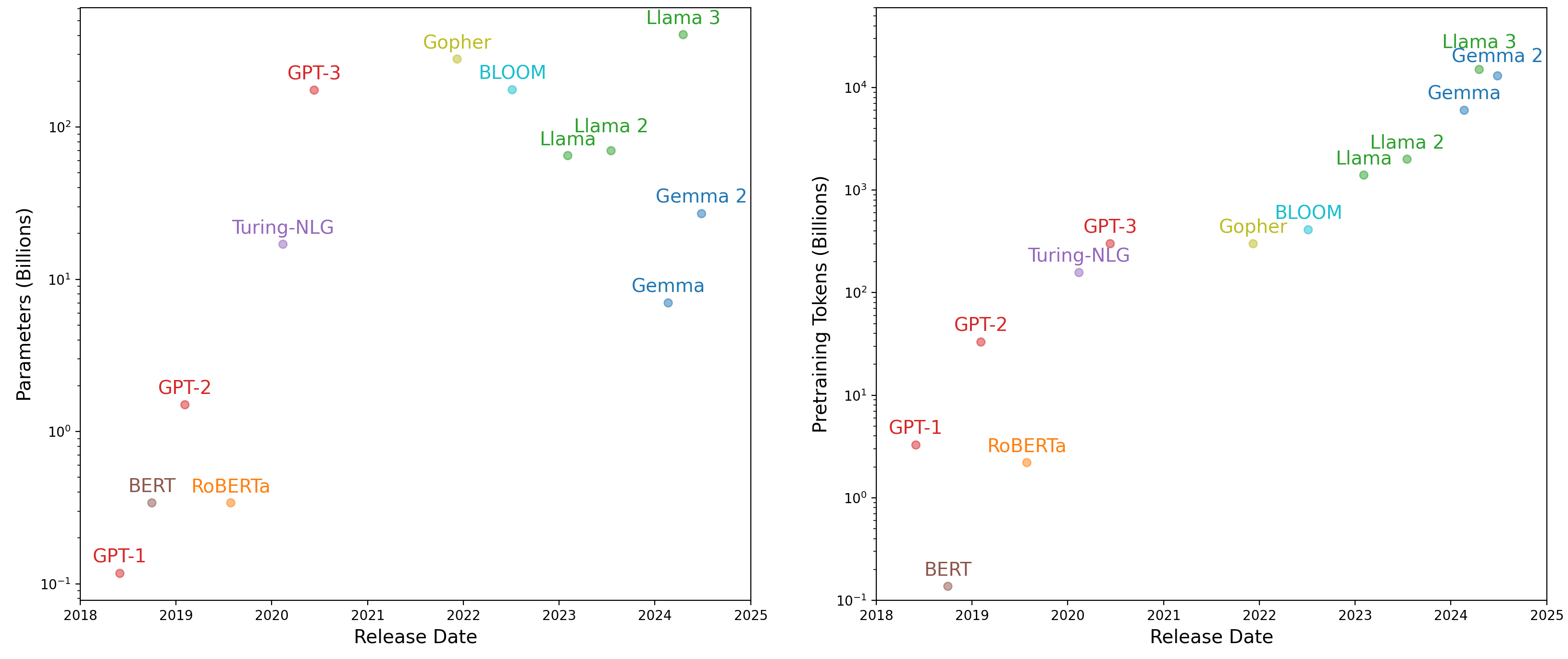
There’s another reason we might not be able to just scale up these models thoughtlessly: we are running out of pretraining data! Tech companies are starting to have trouble finding more high-quality, public, human-written content to throw at pretraining. Models are even beginning to “eat their own tails” by training on a significant portion of content created by other LLMs, which runs into a whole other host of concerns. This is partly why reinforcement learning is getting a lot of attention recently. If you can create a difficult, self-contained environment that generates new problems for an LLM to attempt, you will have found a way to continue training using the model’s own output: no need to scrounge the web for more morsels of quality text.
None of the solutions we touched on will be a silver bullet for the problems facing LLMs. At the end of the day, the fundamental problem remains that LLMs are wildly inefficient at learning compared to humans. Model capabilities come only from training on many orders of magnitude more text than people will read in their lifetimes. As scaling LLMs continues, so will more fundamental research in how to make models that can learn quickly with limited data.
Still, LLMs represent the ability to build fluent, natural language interfaces, and that alone will bring about a massive shift in what we can accomplish with computing devices. In this chapter, we have laid out the basic recipe that many LLMs use to achieve these capabilities.
16.6 Summary
- Large language models, or LLMs, are a combination of a few key ingredients:
- The Transformer architecture
- A language modeling task (predicting the next token based on past tokens)
- A large amount of unlabeled text data
- An LLM learns a probability distribution for predicting individual tokens. This can be combined with a sampling strategy to generate a long string of text. There are many popular ways to sample text:
- Greedy search takes the most likely predicted token at each generation step.
- Random sampling directly samples the predicted categorical distribution over all tokens.
- Top-K sampling restricts the categorical distribution to the top set of
Kcandidates.
- LLMs use billions of parameters and are trained on trillions of words of text.
- LLM output is unreliable, and all LLMs will occasionally hallucinate factually incorrect information.
- LLMs can be fine-tuned to follow instructions in a chat dialog. This type of fine-tuning is called instruction fine-tuning:
- The simplest form of instruction fine-tuning involves directly training the model on instruction and response pairs.
- More advanced forms of instruction fine-tuning involve reinforcement learning.
- The most common resource bottleneck when working with LLMs is accelerator memory.
- LoRA is a technique to reduce memory usage by freezing most Transformer parameters and only updating a low-rank decomposition of attention projection weights.
- LLMs can input or output data from different modalities if you can figure out how to frame these inputs or outputs as sequences in a sequence prediction problem.
- A foundation model is a general term for models, of any modality, trained using self-supervision for a wide range of downstream tasks.
In 2022, Jason Allen used the image generation software Midjourney to win an award for digital artists, and in 2024, Rie Kudan won one of Japan’s most prestigious literary awards for a novel written with substantial help from generative software.↩︎
Iannis Xenakis, “Musiques formelles: nouveaux principes formels de composition musicale,” special issue of La Revue musicale, nos. 253–254 [1963]↩︎
J. Edward Hu et al., “LoRA: Low-Rank Adaptation of Large Language Models,” arXiv [2021], https://arxiv.org/abs/2106.09685.↩︎
Ouyang et al., “Training Language Models to Follow Instructions with Human Feedback,” Proceedings of the 36th International Conference on Neural Information Processing Systems, https://arxiv.org/abs/2203.02155.↩︎