3  Introduction to TensorFlow, PyTorch, JAX, and Keras

This chapter covers

• The major deep learning frameworks and their relationships
• How core deep learning concepts translate to code across all frameworks

This chapter is meant to give you everything you need to start doing deep learning in practice. First you’ll get familiar with three popular deep learning frameworks that can be used with Keras:

• TensorFlow (https://tensorflow.org)
• PyTorch (https://pytorch.org)
• JAX (https://jax.readthedocs.io)

Then, building on your first contact with Keras in chapter 2, we’ll review the core components of neural networks and how they translate to Keras APIs. By the end of this chapter, you’ll be ready to move on to practical, real-world applications starting in chapter 4.

3.1 A brief history of deep learning frameworks

In the real world, you’re not going to be writing low-level code from scratch as we did at the end of chapter 2. Instead, you’re going to use a framework. Besides Keras, the main deep learning frameworks today are JAX, TensorFlow, and PyTorch. This book will teach you about all four.

If you’re just getting started with deep learning, it may seem like all these frameworks have existed forever. In reality, they’re all recent, with Keras being the oldest (launched in March 2015). The ideas behind these frameworks, however, have a long history: the first paper about automatic differentiation was published in 1964¹

All these frameworks combine three key features:

• A way to compute gradients for arbitrary differentiable functions (automatic differentiation)
• A way to run tensor computations on CPUs and GPUs (and possibly even on other specialized deep learning hardware)
• A way to distribute computation across multiple devices in one machine (for example, several GPUs) or across multiple machines

Together, these three simple features unlock all modern deep learning.

It took a long time for the field to develop robust solutions for all three and package those solutions in a reusable form. From its inception in the 1960s through the 2000s, automatic differentiation had no practical applications in machine learning; folks who worked with neural networks simply wrote their own gradient logic by hand, usually in a language like C++. Meanwhile, GPU programming was all but impossible.

Things began to change slowly in the late 2000s. First, Python and its ecosystem were slowly rising in popularity in the scientific community, gaining traction over MATLAB and C++. Second, NVIDIA released CUDA in 2006, unlocking the possibility of building neural networks that could run on consumer GPUs. The initial focus on CUDA was physics simulations rather than machine learning, but that didn’t stop machine learning researchers from implementing CUDA-based neural networks from 2009 onward. They were typically one-off implementations that ran on a single GPU without any automatic differentiation.

The first framework to enable automatic differentiation and GPU computation to train deep learning models was Theano, circa 2009. Theano is the conceptual ancestor of all modern deep learning tools. It gained significant traction in the machine learning research community in 2013–2014, after the results of the ImageNet 2012 competition sparked global interest in deep learning. Around the same time, a few other GPU-enabled deep learning libraries began gaining popularity in the computer vision world—in particular, Torch 7 (Lua-based) and Caffe (C++-based). Keras launched in early 2015 as a higher-level, easier-to-use deep learning library powered by Theano, and it quickly gained traction among the few thousand people who were into deep learning at the time.

Then, in late 2015, Google launched TensorFlow, which took many of the key ideas from Theano and added support for large-scale distributed computation. The release of TensorFlow was a watershed moment that precipitated deep learning in the mainstream developer zeitgeist. Keras immediately added support for TensorFlow. By mid-2016, over half of all TensorFlow users were using it through Keras.

The R interfaces to TensorFlow and Keras were made available in late 2016 and early 2017, respectively. They are principally developed and maintained by Posit PBC (formerly RStudio PBC).

In response to TensorFlow, Meta (then known as Facebook) launched PyTorch about a year later, drawing on ideas from Chainer (a niche but innovative framework launched in mid-2015, now long dead) and NumPy-Autograd, a CPU-only autodifferentiation library for NumPy released by Maclaurin et al. in 2014. Meanwhile, Google released TPUs as an alternative to GPUs, alongside Accelerated Linear Algebra (XLA), a high-performance compiler developed to enable TensorFlow to run on TPUs.

A few years later, at Google, Matthew Johnson—one of the developers who worked on NumPy-Autograd—released JAX as an alternative way to use automatic differentiation with XLA. JAX quickly gained traction with researchers thanks to its minimalistic API and high scalability. Today, Keras, TensorFlow, PyTorch, and JAX are the top frameworks in the deep learning world.

Looking back on this chaotic history, we can ask: What’s next? Will a new framework arise tomorrow? Will we switch to a new programming language or a new hardware platform?

Three things today are certain:

• Python is here to stay. Its machine learning and data science ecosystem has enormous momentum at this point. There won’t be a brand-new language to replace it anytime soon. Note that this isn’t a limitation for R users, because everything in the Python ecosystem can be natively accessed in R through reticulate (more on this later).
• We’re in a multiframework world. All four frameworks are well established and unlikely to go anywhere in the next few years. It’s a good idea for you to learn a little about each one. However, it’s highly possible that new frameworks will gain popularity in the future; Apple’s recently released MLX could be one such example. In this context, using Keras is a considerable advantage: you should be able to run your existing Keras models on any up-and-coming framework via a new Keras backend. Keras will continue to provide future-proof stability to machine learning developers, as it has since 2015—back when TensorFlow, PyTorch, and JAX didn’t exist.
• New chips may be developed in the future, alongside NVIDIA’s GPUs and Google’s TPUs. For instance, AMD’s GPU line likely has bright days ahead. But any such new chips will have to work with the existing frameworks to gain traction. New hardware is unlikely to disrupt your workflows.

3.2 How these frameworks relate to each other

Keras, TensorFlow, PyTorch, and JAX don’t all have the same feature set and aren’t interchangeable. They have some overlap, but to a large extent, they serve different roles for different use cases. The biggest difference is between Keras and the other three. Keras is a high-level framework, whereas the others are lower level. Imagine building a house. Keras is like a prefabricated building kit: it provides a streamlined interface for setting up and training neural networks. In contrast, TensorFlow, PyTorch, and JAX are like the raw materials used in construction.

As you saw in the previous chapters, training a neural network revolves around the following concepts:

• Low-level tensor manipulation—the infrastructure that underlies all modern machine learning. This translates to low-level APIs found in TensorFlow, PyTorch, and JAX. (PyTorch is an intermediate case: although it is mainly a lower-level framework, it also includes its own layers and optimizers. However, if you use PyTorch in conjunction with Keras, you will only interact with low-level PyTorch APIs such as tensor operations.)
  • Tensors, including special tensors that store the network’s state (variables)
  • Tensor operations such as addition, relu, and matmul
  • Backpropagation, a way to compute the gradient of mathematical expressions
• High-level deep learning concepts. This translates to Keras APIs:
  • Layers, which are combined into a model
  • A loss function, which defines the feedback signal used for learning
  • An optimizer, which determines how learning proceeds
  • Metrics to evaluate model performance, such as accuracy
  • A training loop that performs mini-batch stochastic gradient descent

Further, Keras is unique in that it isn’t a fully standalone framework. It needs a backend engine to run, much as a prefabricated house-building kit needs to source building materials. TensorFlow, PyTorch, and JAX can all be used as Keras backends. In addition, Keras can run on NumPy; but because NumPy does not provide an API for gradients, Keras workflows on NumPy are restricted to making predictions from a model—training is impossible.

Now that you have a clearer understanding of how all these frameworks and interfaces came to be and how they relate to each other, let’s dive into what it’s like to work with them. We’ll cover them in chronological order: TensorFlow first, then PyTorch, and finally JAX.

View on GitHub Run on Colab

3.3 Introduction to TensorFlow

TensorFlow is a Python-based open source machine learning framework developed primarily by Google. Its initial release was in November 2015, followed by a v1 release in February 2017 and a v2 release in October 2019. TensorFlow is heavily used in production-grade machine learning applications across the industry.

It’s important to keep in mind that TensorFlow is more than a single library. It’s a platform, home to a vast ecosystem of components, some developed by Google and others by third parties. For instance, there’s TFX for industry-strength machine learning workflow management, TF-Serving for production deployment, the TF Optimization Toolkit for model quantization and pruning, and TFLite and MediaPipe for mobile application deployment. Together, these components cover a very wide range of use cases, from cutting-edge research to large-scale production applications.

3.3.1 First steps with TensorFlow

In this section, you’ll get familiar with the basics of TensorFlow. We’ll cover the following key concepts:

• Tensors and variables
• Numerical operations in TensorFlow
• Computing gradients with GradientTape
• Making TensorFlow functions fast by using just-in-time compilation

We’ll conclude the introduction with an end-to-end example: a pure-TensorFlow implementation of a linear classifier.

Let’s get those tensors flowing:

library(tensorflow)
library(keras3)
use_backend("tensorflow")

NoteUsing Python modules in R

The tensorflow R package makes the tensorflow Python module directly available. Calling tf.ones() in Python is identical to calling tf$ones() in R.

Generally, we can call TensorFlow functions as regular R functions without any special handling. These are a few things to keep in mind:

• Python uses zero-based indexing (e.g., in functions like tf.slice()).
• You can consult the Python documentation directly: everything there applies. The TensorFlow R package installs a help handler that integrates with the RStudio IDE. For example, pressing F1 while the cursor is on tf$ones will open the corresponding Python documentation. The R print method for a Python callable will show the function signature, and you can also view the built-in Python help page with py_help(tf$ones).
• In R, bare numbers like 1 are doubles by default, whereas in Python they’re integers. This can cause issues if a Python function expects an integer. To create an integer in R, append an L, as in 1L.
• Some Python functions expect specific container types, like tuples (similar to unnamed lists in R). We can create a tuple in R using tuple().

The need for a tuple of integers comes up often when specifying a tensor shape. For convenience, keras3 provides shape(), which returns an object that converts to a tuple of integers when passed to Python functions.

3.3.1.1 Tensors and variables in TensorFlow

To do anything in TensorFlow, we need some tensors. There are a few different ways to create them.

3.3.1.1.1 Constant tensors

Tensors need to be created with an initial value, so common ways to create tensors are via tf$ones() and tf$zeros(). We can also create a tensor from R or NumPy values using tf$constant():

tf$ones(shape = shape(2, 2))

tf.Tensor(
[[1. 1.]
 [1. 1.]], shape=(2, 2), dtype=float32)

tf$zeros(shape = shape(2, 2))

tf.Tensor(
[[0. 0.]
 [0. 0.]], shape=(2, 2), dtype=float32)

tf$constant(c(1, 2, 3), dtype = "float32")

tf.Tensor([1. 2. 3.], shape=(3), dtype=float32)

3.3.1.1.2 Random tensors

We can create tensors filled with random values via one of the functions in the tf$random submodule:

1tf$random$normal(shape(3, 1), mean = 0, stddev = 1)

1

Tensor of random values drawn from a normal distribution with mean 0 and standard deviation 1

tf.Tensor(
[[-0.05340578]
 [-0.8541691 ]
 [ 0.9360311 ]], shape=(3, 1), dtype=float32)

1tf$random$uniform(shape(3, 1), minval = 0, maxval = 1)

1

Tensor of random values drawn from a uniform distribution between 0 and 1

tf.Tensor(
[[0.93514407]
 [0.73917115]
 [0.8291607 ]], shape=(3, 1), dtype=float32)

3.3.1.1.3 Tensor assignment and the Variable class

A significant difference between NumPy arrays and TensorFlow tensors is that TensorFlow tensors aren’t assignable: they’re constant. For instance, with an R array or NumPy array, we can do the following:

x <- array(1, dim = c(2, 2))
x[1, 1] <- 0

If we try to do the same thing in TensorFlow, we will get an error—"EagerTensor object does not support item assignment":

x <- tf$ones(shape(2, 2))
1x@r[1, 1] <- 0.

1

This will fail, as a tensor isn’t assignable.

Error in `py_set_item()`:
! TypeError: 'tensorflow.python.framework.ops.EagerTensor' object does not support item assignment
Run `reticulate::py_last_error()` for details.

To train a model, we need to update its state, which is a set of tensors. If tensors aren’t assignable, how do we do that? This is where variables come in. tf$Variable is the class meant to manage modifiable state in TensorFlow.

To create a variable, we need to provide an initial value, such as a tensor of random values or of zeros:

v <- tf$Variable(initial_value = tf$zeros(shape = shape(3, 1)))
v

<tf.Variable 'Variable:0' shape=(3, 1) dtype=float32, numpy=
array([[0.],
       [0.],
       [0.]], dtype=float32)>

The state of a variable can be modified via its $assign() method:

v$assign(tf$ones(shape(3, 1)))
v

<tf.Variable 'Variable:0' shape=(3, 1) dtype=float32, numpy=
array([[1.],
       [1.],
       [1.]], dtype=float32)>

The @r[<- method is convenient shorthand for calling assign():

v@r[] <- tf$zeros(shape(3, 1))
v

<tf.Variable 'UnreadVariable' shape=(3, 1) dtype=float32, numpy=
array([[0.],
       [0.],
       [0.]], dtype=float32)>

Assignment also works for a subset of the coefficients:

v@r[1, 1]$assign(3)
v@r[2, 1] <- 4
v

<tf.Variable 'UnreadVariable' shape=(3, 1) dtype=float32, numpy=
array([[3.],
       [4.],
       [0.]], dtype=float32)>

Similarly, assign_add and assign_sub are efficient equivalents of the v <- v + y and v <- v - y operations:

v$assign_add(tf$ones(shape(3, 1)))
v

<tf.Variable 'UnreadVariable' shape=(3, 1) dtype=float32, numpy=
array([[4.],
       [5.],
       [1.]], dtype=float32)>

3.3.1.2 Tensor operations: Doing math in TensorFlow

Like any mature numerical computing environment, TensorFlow offers a large collection of tensor operations to express mathematical formulas. Here are a few examples:

a <- tf$ones(shape(2, 2))
1b <- tf$square(a)
2c <- tf$sqrt(a)
3d <- b + c
4e <- tf$matmul(a, b)
5f <- tf$concat(list(a, b), axis = 0L)

1

Takes the square, the same as a*a or a^2

2

Takes the square root, the same as sqrt

3

Adds two tensors (element-wise)

4

Takes the product of two tensors (see chapter 2), the same as %*%

5

Concatenates a and b along the first axis. tf$concat() is a generalized version of cbind() and rbind() for nd-arrays. Note that axis is 0-based!

Here’s an equivalent of the Dense layer we saw in chapter 2:

dense <- function(inputs, W, b) {
  tf$nn$relu(tf$matmul(inputs, W) + b)
}

3.3.1.3 Gradients in TensorFlow: A second look at the GradientTape API

So far, TensorFlow looks a lot like NumPy. But here’s something NumPy (or base R) can’t do: retrieve the gradient of any differentiable expression with respect to any of its inputs. Just open a GradientTape scope, apply some computation to one or several input tensors, and retrieve the gradient of the result with respect to the inputs:

input_var <- tf$Variable(initial_value = 3)
with(tf$GradientTape() %as% tape, {
  result <- tf$square(input_var)
})
gradient <- tape$gradient(result, input_var)

This technique is most commonly used to retrieve the gradients of the loss of a model with respect to its weights: gradients <- tape$gradient(loss, weights).

In chapter 2, you saw that GradientTape works on either a single input or a list of inputs and that inputs can be either scalars or high-dimensional tensors.

So far, you’ve only seen the case where the input tensors in tape$gradient() are TensorFlow variables. It’s possible for these inputs to be any arbitrary tensor; however, only trainable variables are tracked by default. With a constant tensor, we’d have to manually mark it as being tracked by calling tape$watch() on it:

input_const <- tf$constant(3)
with(tf$GradientTape() %as% tape, {
  tape$watch(input_const)
  result <- tf$square(input_const)
})
gradient <- tape$gradient(result, input_const)

Why? Because it would be too expensive to preemptively store the information required to compute the gradient of anything with respect to anything. To avoid wasting resources, the tape needs to know what to watch. Trainable variables are watched by default because computing the gradient of a loss with regard to a list of trainable variables is the most common use case of the gradient tape.

The gradient tape is a powerful utility that can even compute second-order gradients—that is, the gradient of a gradient. For instance, the gradient of the position of an object with regard to time is the speed of that object, and the second-order gradient is its acceleration.

If we measure the position of a falling apple along a vertical axis over time and find that it verifies position(time) = 4.9 * time^2, what is its acceleration? Let’s use two nested gradient tapes to find out:

time <- tf$Variable(0)
with(tf$GradientTape() %as% outer_tape, {
  with(tf$GradientTape() %as% inner_tape, {
    position <- 4.9 * time^2
  })
  speed <- inner_tape$gradient(position, time)
})
1acceleration <- outer_tape$gradient(speed, time)
acceleration

1

We use the outer tape to compute the gradient of the gradient from the inner tape. Naturally, the answer is 4.9 * 2 = 9.8.

tf.Tensor(9.8, shape=(), dtype=float32)

3.3.1.4 Making TensorFlow functions fast using compilation

All the TensorFlow code you’ve written so far has been executing “eagerly.” This means operations are executed one after the other in the R runtime, much like any non-lazy R code or NumPy code. Eager execution is great for debugging, but it is typically slow. It can often be beneficial to parallelize computation or “fuse” operations: replacing two consecutive operations, like matmul followed by relu, with a single, more efficient operation that does the same thing without materializing the intermediate output.

This can be achieved via compilation. The general idea of compilation is to take certain functions you’ve written in R, lift them out of R (and Python), automatically rewrite them into a faster and more efficient “compiled program,” and then call that program from the R runtime.

The main benefit of compilation is improved performance. There’s a drawback, too: the code we write is no longer the code that gets executed, which can make the debugging experience painful. Only turn on compilation after you’ve already debugged your code in the R runtime.

We can apply compilation to any TensorFlow function by wrapping it with tf_function(), like this:

dense <- tf_function(\(inputs, W, b) {
  tf$nn$relu(tf$matmul(inputs, W) + b)
})

When we do this, any call to dense() is replaced with a call to a compiled program that implements a more optimized version of the function. The first call to the function will take longer, because TensorFlow will be compiling our code. This only happens once: all subsequent calls to the same function will be fast.

TensorFlow has two compilation modes:

• The default, which we refer to as graph mode. Any function decorated with tf_function() runs in graph mode.
• Compilation with XLA, a high-performance compiler for ML. We turn it on by specifying jit_compile = TRUE, like this:

dense <- tf_function(jit_compile = TRUE, \(inputs, W, b) {
  tf$nn$relu(tf$matmul(inputs, W) + b)
})

Compiling a function with XLA will often make it run faster than graph mode. However, executing the function the first time takes longer because the compiler has more work to do.

3.3.2 An end-to-end example: A linear classifier in pure TensorFlow

You know about tensors, variables, and tensor operations, and you know how to compute gradients. That’s enough to build any TensorFlow-based machine learning model based on gradient descent. Let’s walk through an end-to-end example to make sure everything is crystal clear.

In a machine learning job interview, you may be asked to implement a linear classifier from scratch. This is a very simple task that serves as a filter between candidates who have some minimal machine learning background and those who don’t. Let’s get you past that filter and use your newfound knowledge of TensorFlow to implement such a linear classifier.

First, let’s come up with some nicely linearly separable synthetic data to work with—two classes of points in a 2D plane:

num_samples_per_class <- 1000
Sigma <- rbind(c(1, 0.5),
               c(0.5, 1))
1negative_samples <- MASS::mvrnorm(
  n = num_samples_per_class,
  mu = c(0, 3),
  Sigma = Sigma
)
2positive_samples <- MASS::mvrnorm(
  n = num_samples_per_class,
  mu = c(3, 0),
  Sigma = Sigma
)

1

Generates the first class of points: 1,000 random 2D points with specified mean and covariance matrix. Intuitively, the covariance matrix describes the shape of the point cloud and the mean describes its position in the plane. Sigma corresponds to an oval-like point cloud oriented from bottom left to top right.

2

Generates the other class of points with a different mean and the same covariance matrix (point cloud with a different position and the same shape)

negative_samples and positive_samples are both arrays with shape (1000, 2). Let’s stack them into a single array with shape (2000, 2):

inputs <- rbind(negative_samples, positive_samples)

Let’s generate the corresponding target labels. They are in an array of zeros and ones of shape (2000, 1), where targets[i, 1] is 0 if inputs[i] belongs to class 0 and 1 if it belongs to class 1:

targets <- rbind(array(0, dim = c(num_samples_per_class, 1)),
                 array(1, dim = c(num_samples_per_class, 1)))

Let’s plot our data (see figure 3.1):

plot(x = inputs[, 1], y = inputs[, 2],
     col = ifelse(targets[, 1] == 0, "purple", "green"))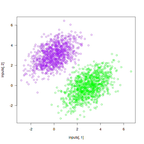

Our synthetic data: two classes of random points in the 2D plane

Now, let’s create a linear classifier that can learn to separate these two blobs. A linear classifier is an affine transformation (prediction = matmul(input, W) + b) trained to minimize the square of the difference between predictions and the targets.

As you’ll see, this is a much simpler example than the end-to-end example of a toy two-layer neural network from the end of chapter 2. However, this time you should be able to understand everything about the code, line by line.

Let’s create our variables W and b, initialized with random values and with zeros, respectively:

1input_dim <- 2
2output_dim <- 1
W <- tf$Variable(
  initial_value = tf$random$uniform(shape(input_dim, output_dim))
)
b <- tf$Variable(
  initial_value = tf$zeros(shape(output_dim))
)

1

The inputs will be 2D points.

2

The output predictions will be a single score per sample (close to 0 if the sample is predicted to be in class 0, and close to 1 if the sample is predicted to be in class 1).

Here’s our forward pass function:

model <- function(inputs, W, b) {
  tf$matmul(inputs, W) + b
}

Because our linear classifier operates on 2D inputs, W is really two scalar coefficients: W = [[w1], [w2]]. Meanwhile, b is a single scalar coefficient. As such, for a given input point [x, y], its prediction value is prediction = [[w1], [w2]] • [x, y] + b = w1 * x + w2 * y + b.

Here’s our loss function:

mean_squared_error <- function(targets, predictions) {
1  per_sample_losses <- tf$square(targets - predictions)
2  tf$reduce_mean(per_sample_losses)
}

1

per_sample_losses will be a tensor with the same shape as targets and predictions, containing per-sample loss scores

2

Averages these per-sample loss scores into a single scalar loss value

Now we move to the training step, which receives some training data and updates the weights W and b to minimize the loss on the data:

learning_rate <- 0.1

1training_step <- tf_function(
  jit_compile = TRUE,
  \(inputs, targets, W, b) {
    with(tf$GradientTape() %as% tape, {
2      predictions <- model(inputs, W, b)
      loss <- mean_squared_error(targets, predictions)
    })
3    grad_loss_wrt <- tape$gradient(loss, list(W = W, b = b))
4    W$assign_sub(grad_loss_wrt$W * learning_rate)
    b$assign_sub(grad_loss_wrt$b * learning_rate)
    loss
  }
)

1

Wrap the function with tf_function() to speed it up

2

Forward pass, inside of a gradient tape scope

3

Retrieve the gradient of the loss with regard to weights

4

Update the weights

For simplicity, we’ll do batch training instead of mini-batch training: we’ll run each training step (gradient computation and weight update) on all of the data rather than iterating over the data in small batches. On one hand, this means that each training step will take much longer to run, because we compute the forward pass and the gradients for 2,000 samples at once. On the other hand, each gradient update will be much more effective at reducing the loss on the training data, because it will encompass information from all training samples instead of, say, only 128 random samples. As a result, we will need many fewer steps of training, and we should use a larger learning rate than we would typically use for mini-batch training (we’ll use learning_rate <- 0.1, as previously defined):

inputs <- np_array(inputs, dtype = "float32")
targets <- np_array(targets, dtype = "float32")

for (step in 1:40) {
  loss <- training_step(inputs, targets, W, b)
  if (step < 5 || !step %% 5)
    cat(sprintf("Loss at step %d: %.4f\n", step, loss))
}

Loss at step 1: 4.5364
Loss at step 2: 0.4348
Loss at step 3: 0.1636
Loss at step 4: 0.1271
Loss at step 5: 0.1155
Loss at step 10: 0.0816
Loss at step 15: 0.0606
Loss at step 20: 0.0475
Loss at step 25: 0.0393
Loss at step 30: 0.0341
Loss at step 35: 0.0309
Loss at step 40: 0.0289

After 40 steps, the training loss seems to have stabilized at around 0.028. Let’s plot how our linear model classifies the training data points, as shown in figure 3.2. Because our targets are zeros and ones, a given input point will be classified as “0” if its prediction value is below 0.5, and as “1” if it is above 0.5. Note that figure 3.2 looks very similar to figure 3.1 because the model learns to separate the two classes well, but it is not a duplicate: figure 3.1 is colored based on the true targets, whereas figure 3.2 is colored based on the model’s predicted classes.

predictions <- model(inputs, W, b)

1predictions <- as.array(predictions)
inputs <- as.array(inputs)
targets <- as.array(targets)

plot(x = inputs[, 1], y = inputs[, 2],
     col = ifelse(predictions[, 1] > 0.5, "green", "purple"))

1

Converts tensors to R arrays

Our model’s predictions on the training inputs: pretty similar to the training targets

Recall that the prediction value for a given point [x, y] is simply prediction = [[w1], [w2]] • [x, y] + b = w1 * x + w2 * y + b. Thus, class “0” is defined as w1 * x + w2 * y + b < 0.5 and class “1” is defined as w1 * x + w2 * y + b > 0.5. Notice that this is the equation of a line in the 2D plane: w1 * x + w2 * y + b = 0.5. Class 1 is above the line; class 0 is below the line. You may be used to seeing line equations in the format y = a * x + b; in the same format, our line becomes y = - w1 / w2 * x + (0.5 - b) / w2.

Let’s plot this line (see figure 3.3):

plot(x = inputs[, 1], y = inputs[, 2],
     col = ifelse(predictions[, 1] <= 0.5, "purple", "green"))

slope <- -W[1, ] / W[2, ]
intercept <- (0.5 - b) / W[2, ]
abline(as.array(intercept), as.array(slope), col = "red")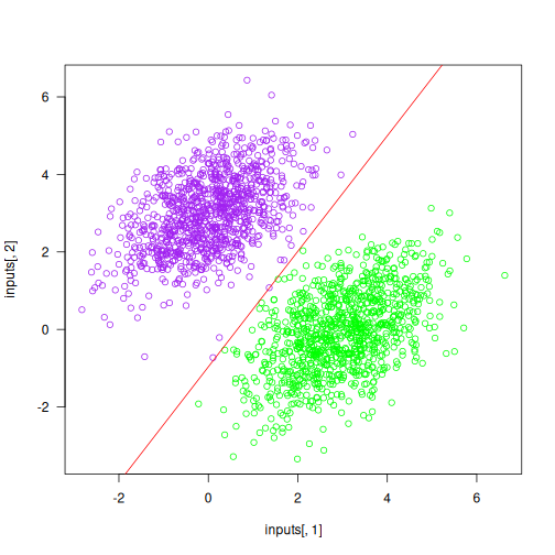

Our model, visualized as a line

This is what a linear classifier is all about: finding the parameters of a line (or, in higher-dimensional spaces, a hyperplane) that neatly separates two classes of data.

3.3.3 What makes the TensorFlow approach unique

You’re now familiar with all the basic APIs that underlie TensorFlow-based workflows. What makes working with TensorFlow different from working with any other framework? When should you use TensorFlow, and when should you use something else?

Here are the main benefits of TensorFlow:

• Thanks to graph mode and XLA compilation, it’s fast. It’s usually significantly faster than PyTorch and NumPy, although JAX is often even faster.
• It is extremely feature-complete. Unique among all frameworks, it has support for string tensors as well as “ragged tensors” (tensors where different entries may have different dimensions—very useful for handling sequences without requiring them to be padded to a shared length). It also has outstanding support for data preprocessing, via the highly performant tf.data API. tf.data is so good that even JAX recommends it for data preprocessing. Whatever we need to do, TensorFlow has a solution for it.
• Its ecosystem for production deployment is the most mature among all frameworks, especially when it comes to deploying on mobile or in the browser.

However, TensorFlow also has some noticeable flaws:

• It has a sprawling API—the flipside of being very feature-complete. TensorFlow includes thousands of different operations.
• Its numerical API is occasionally inconsistent with the NumPy API, making it harder to approach if you’re already familiar with NumPy.
• The popular pretrained model-sharing platform Hugging Face has less support for TensorFlow, which means the latest generative AI models may not always be available in TensorFlow.

Now, let’s move on to PyTorch.

View on GitHub Run on Colab

3.4 Introduction to PyTorch

PyTorch is a Python-based open source machine learning framework developed primarily by Meta (formerly Facebook). It was originally released in September 2016 (as a response to the release of TensorFlow), with its 1.0 version launched in 2018 and its 2.0 version launched in 2023. PyTorch is used extensively in the machine learning research community.

Like TensorFlow, PyTorch is at the center of a large ecosystem of related packages, such as torchvision, torchaudio, and the popular model-sharing platform Hugging Face. The PyTorch API is higher level than that of TensorFlow and JAX: it includes layers and optimizers, like Keras. However, when we use Keras with the PyTorch backend, we’ll primarily use Keras layers and optimizers and only interact with low-level PyTorch APIs such as tensor operations.

3.4.1 First steps with PyTorch

This section covers the following key concepts:

• Tensors and parameters
• Numerical operations in PyTorch
• Computing gradients with the backward() method
• Packaging computation with the Module class
• Speeding up PyTorch by using compilation

We’ll conclude the introduction by reimplementing our linear classifier end-to-end example in pure PyTorch.

3.4.1.1 Tensors and parameters in PyTorch

To use PyTorch, start an R session as follows (only one Keras backend can be used per R session):

library(keras3)
use_backend("torch")

torch <- import("torch")

NoteUsing reticulate

We accessed TensorFlow via the tensorflow R package. However, for PyTorch and JAX, we use reticulate::import() to access the Python module. This might make it seem like these are two different approaches—but they’re not!

The tf object from the tensorflow R package is the same object we get by calling reticulate::import("tensorflow").

The Python ecosystem is enormous, and reticulate provides direct access to all of it.

A first gotcha about PyTorch is that the package isn’t named pytorch: it’s named torch. Note that this is different from the R package named torch! In a self-managed Python installation, we’d install it with pip install torch. In R, we can declare it as a Python requirement with py_require("torch") and import it via import("torch") (but usually we don’t have to do that if we’re using keras3::use_backend("torch")).

As with TensorFlow, the object at the heart of the framework is the tensor. Let’s get our hands on some PyTorch tensors.

3.4.1.1.1 Constant tensors

Here are some constant tensors:

1torch$ones(size = shape(2, 2))

1

Unlike in other frameworks, the shape argument is named “size” rather than “shape.”

tensor([[1., 1.],
        [1., 1.]])

torch$zeros(size = shape(2, 2))

tensor([[0., 0.],
        [0., 0.]])

1torch$tensor(c(1, 2, 3), dtype = torch$float32)

1

Unlike in other frameworks, we cannot pass dtype=“float32” as a string. The dtype argument must be a torch dtype instance.

tensor([1., 2., 3.])

3.4.1.1.2 Random tensors

Random tensor creation is similar to in NumPy and TensorFlow, but with divergent syntax. Consider the function normal: it doesn’t take a shape argument. Instead, the mean and standard deviation should be provided as PyTorch tensors with the expected output shape:

1torch$normal(
  mean = torch$zeros(size = shape(1, 3)),
  std = torch$ones(size = shape(1, 3))
)

1

Equivalent to tf$random$normal(shape(1, 3), mean=0, stddev=1)

tensor([[ 0.2692, -1.3085, -0.8149]])

We’d create a random uniform tensor via torch$rand(). Unlike tf.random.uniform(), the output shape should be provided via independent arguments for each dimension, like this:

1torch$rand(1L, 3L)

1

Equivalent to tf$random$uniform(shape(1, 3), minval=0, maxval=1)

tensor([[0.6361, 0.6597, 0.8087]])

We can still use the shape() convenience function if we pair it with the dots splicing operator from rlang (which is supported for all reticulated Python functions):

torch$rand(!!!shape(1, 3))

tensor([[0.4713, 0.9026, 0.3267]])

3.4.1.1.3 Tensor assignment and the Parameter class

Unlike TensorFlow tensors, but like NumPy arrays, PyTorch tensors can be modified in place. We can do operations like this:

x <- torch$zeros(size = shape(2, 2))
x@py[0, 0] <- 1
x

tensor([[1., 0.],
        [0., 0.]])

Although we can use a regular torch$Tensor to store the trainable state of a model, PyTorch provides a specialized tensor subclass for that purpose: the torch$nn$parameter$Parameter class. Compared to a regular tensor, it provides semantic clarity: if we see a Parameter, we know it’s a piece of trainable state, whereas a Tensor could be anything. As a result, PyTorch can automatically track and retrieve the Parameters we assign to PyTorch models, similar to what Keras does with Keras Variable instances.

Here’s a Parameter:

x <- torch$zeros(shape(2, 1))
1p <- torch$nn$parameter$Parameter(data = x)

1

A Parameter can only be created using a torch.Tensor value—no NumPy or R arrays allowed.

3.4.1.2 Tensor operations: Doing math in PyTorch

Math in PyTorch works just the same as math in NumPy or TensorFlow, although much like TensorFlow, the PyTorch API often diverges in subtle ways from the NumPy API:

a <- torch$ones(shape(2, 2))
1b <- torch$square(a)
2c <- torch$sqrt(a)
3d <- b + c
4e <- torch$matmul(a, b)
5f <- torch$cat(list(a, b), dim = 0L)

1

Takes the square, the same as a*a or a^2

2

Takes the square root, the same as sqrt()

3

Adds two tensors (element-wise)

4

Takes the product of two tensors (see chapter 2)

5

Concatenates a and b along the first axis

Here’s a dense layer:

dense <- function(inputs, W, b) {
  torch$nn$relu(torch$matmul(inputs, W) + b)
}

3.4.1.3 Computing gradients with PyTorch

There’s no explicit “gradient tape” in PyTorch. A similar mechanism does exist: when we run any computation in PyTorch, the framework creates a one-time computation graph (a tape) that records what just happened. However, that tape is hidden from the user. The public API for using it is at the level of tensors themselves: we can call tensor$backward() to run backpropagation through all operations previously executed that led to that tensor. Doing this will populate the $grad attribute of all tensors that are tracking gradients:

1input_var <- torch$tensor(3.0, requires_grad = TRUE)
result <- torch$square(input_var)
2result$backward()
gradient <- input_var$grad
gradient

1

To compute gradients with respect to a tensor, it must be created with requires_grad=TRUE.

2

Calling backward() populates the “grad” attribute on all tensors created with requires_grad=TRUE.

If you call backward() multiple times in a row, the $grad attribute will “accumulate” gradients: each new call will sum the new gradient with the preexisting one. For instance, in the following code, input_var$grad is not the gradient of square(input_var) with respect to input_var; rather, it is the sum of that gradient and the previously computed gradient—its value has doubled since our last code snippet:

tensor(6.)

result <- torch$square(input_var)
result$backward()
1input_var$grad

1

$grad will sum all gradient values from each time backward() is called.

tensor(12.)

To reset gradients, we can set $grad to NULL:

input_var$grad <- NULL

Now let’s put this into practice!

3.4.2 An end-to-end example: A linear classifier in pure PyTorch

You now know enough to rewrite our linear classifier in PyTorch. It will be very similar to the TensorFlow one—the only major difference is how we compute the gradients.

Let’s start by creating our model variables. Don’t forget to pass requires_grad=TRUE so you can compute gradients with respect to them:

input_dim <- 2L
output_dim <- 1L

W <- torch$rand(input_dim, output_dim, requires_grad = TRUE)
b <- torch$zeros(output_dim, requires_grad = TRUE)

This is our model—no difference so far. We just went from tf$matmul() to torch$matmul():

model <- function(inputs, W, b) {
  torch$matmul(inputs, W) + b
}

This is our loss function. We switch from tf$square() to torch$square() and from tf$reduce_mean() to torch$mean():

mean_squared_error <- function(targets, predictions) {
  per_sample_losses <- torch$square(targets - predictions)
  torch$mean(per_sample_losses)
}

Now for the training step. Here’s how it works:

1. loss$backward() runs backpropagation starting from the loss output node and populates the tensor$grad attribute on all tensors that were involved in the computation of loss. tensor$grad represents the gradient of the loss with regard to that tensor.
2. We use the $grad attribute to recover the gradients of the loss with regard to W and b.
3. We update W and b using those gradients. Because these updates are not intended to be part of the backwards pass, we do them inside a torch$no_grad() scope, which skips gradient computation for everything inside it.
4. We reset the contents of the $grad property of our W and b parameters, by setting it to NULL. If we didn’t do this, gradient values would accumulate across multiple calls to training_step(), resulting in invalid values.

Here’s the code:

learning_rate <- 0.1

training_step <- function(inputs, targets, W, b) {
1  predictions <- model(inputs, W, b)
  loss <- mean_squared_error(targets, predictions)
2  loss$backward()
3  grad_loss_wrt_W <- W$grad
  grad_loss_wrt_b <- b$grad
  with(torch$no_grad(), {
4    W$sub_(grad_loss_wrt_W * learning_rate)
    b$sub_(grad_loss_wrt_b * learning_rate)
  })
5  W$grad <- b$grad <- NULL
  loss
}

1

Forward pass

2

Computes gradients

3

Retrieves gradients

4

Updates weights inside a no_grad scope

5

Resets gradients

This can be made even simpler; let’s see how.

3.4.2.1 Packaging state and computation with the Module class

PyTorch also has a higher-level, object-oriented API for performing backpropagation, which relies on two new classes: the torch$nn$Module class and an optimizer class from the torch$optim module, such as torch$optim$SGD (the equivalent of Keras’s optimizer_sgd()).

The general idea is to define a subclass of torch$nn$Module, which will

• Hold some Parameters to store state variables, defined in the __init__() method
• Implement the forward pass computation in the forward() method.

It should look like the following:

LinearModel(torch$nn$Module) %py_class% {
  `__init__` <- function(self) {
    super()$`__init__`()
    self$W <- torch$nn$Parameter(torch$rand(input_dim, output_dim))
    self$b <- torch$nn$Parameter(torch$zeros(output_dim))
  }
  forward <- function(self, inputs) {
    torch$matmul(inputs, self$W) + self$b
  }
}

We can now instantiate our LinearModel:

model <- LinearModel()

When using an instance of torch$nn$Module, rather than calling the forward() method directly, we use __call__() (i.e., call the model class directly on inputs), which redirects to forward() but adds a few framework hooks to it:

torch_inputs <- torch$tensor(inputs, dtype = torch$float32)
output <- model(torch_inputs)

Now, let’s get our hands on a PyTorch optimizer. To instantiate it, we need to provide the list of parameters that the optimizer is intended to update. We can retrieve it from our Module instance via $parameters():

optimizer <- torch$optim$SGD(model$parameters(), lr = learning_rate)

Using our Module instance and the PyTorch SGD optimizer, we can run a simplified training step:

training_step <- function(inputs, targets) {
  predictions <- model(inputs)
  loss <- mean_squared_error(targets, predictions)
  loss$backward()
  optimizer$step()
  model$zero_grad()
  loss
}

Previously, updating the model parameters looked like this:

with(torch$no_grad(), {
1  W$sub_(grad_loss_wrt_W * learning_rate)
  b$sub_(grad_loss_wrt_b * learning_rate)
})

1

The underscore suffix in sub_ means that W will be modified in place.

Now we can just use optimizer$step().

Similarly, previously we needed to reset parameter gradients by hand by using tensor$grad <- NULL on each one. Now we can just use model$zero_grad().

Overall, this may feel confusing: somehow the loss tensor, the optimizer, and the Module instance all seem to be aware of each other through a hidden background mechanism. They’re all interacting with one another via spooky action at a distance. Don’t worry, though: we can treat this sequence of steps (loss$backward() - optimizer$step() - model$zero_grad()) as a magic incantation to be recited any time we need to write a training step function. Just be sure not to forget model$zero_grad(). That would be a major bug (and is unfortunately common)!

3.4.2.2 Making PyTorch modules fast using compilation

One last thing. Similar to how TensorFlow lets us compile functions for better performance, PyTorch lets us compile functions or even Module instances via the torch$compile() utility. This API uses PyTorch’s very own compiler, named Dynamo.

Let’s try it on our linear classifier Module:

compiled_model <- torch$compile(model)

The resulting object is intended to work identically to the original—except that the forward and backward passes should run faster.

We can also use torch$compile() as a function decorator:

dense <- torch$compile(function(inputs, W, b) {
  torch$nn$relu(torch$matmul(inputs, W) + b)
})

In practice, most PyTorch code does not use compilation and simply runs eagerly, as the compiler may not always work with all models and may not always result in a speedup when it does work. Unlike in TensorFlow and Jax, where compilation was built in from the inception of the library, PyTorch’s compiler is a relatively recent addition.

3.4.3 What makes the PyTorch approach unique

Compared to TensorFlow and JAX, which we will cover next, what makes PyTorch stand out? Why should we use it or not use it?

Here are PyTorch’s two key strengths:

• PyTorch code executes eagerly by default, making it easy to debug. Note that this is also the case for TensorFlow code and JAX code, but a big difference is that PyTorch is generally intended to be run eagerly at all times; any serious TensorFlow or JAX project will inevitably need compilation at some point, which can significantly hurt the debugging experience.
• The popular pretrained model-sharing platform Hugging Face has first-class support for PyTorch, which means that any model we’d like to use is likely available in PyTorch. This is the primary driver behind PyTorch adoption today.

Meanwhile, there are also some downsides to using PyTorch:

• Due to its focus on eager execution, PyTorch is slow: it’s the slowest of all the major frameworks by a large margin. For most models, we may see a 20% or 30% speedup with JAX. For some models—especially large ones—we may see a 3× or 5× speedup with JAX, even after using torch$compile().
• As with TensorFlow, the PyTorch API is inconsistent with NumPy. It’s also internally inconsistent. For instance, the commonly used keyword axis is occasionally named dim instead, depending on the function. Some pseudo-random number generation operations take a seed argument, others don’t; and so on. This can make PyTorch frustrating to learn, especially when coming from NumPy.
• Although it is possible to make PyTorch code faster via torch$compile(), at the time of this writing the PyTorch Dynamo compiler remains ineffective and full of trapdoors. As a result, only a very small percentage of the PyTorch user base uses compilation. Perhaps this will be improved in future versions!

View on GitHub Run on Colab

3.5 Introduction to JAX

JAX is an open source library for differentiable computation, primarily developed by Google. After its release in 2018, JAX quickly gained traction in the research community, particularly for its ability to use Google’s TPUs at scale. Today, JAX is in use by most of the top players in the generative AI space: companies like DeepMind, Apple, Midjourney, Anthropic, Cohere, and so on.

JAX embraces a stateless approach to computation, meaning that functions in JAX do not maintain any persistent state. This contrasts with traditional Python imperative programming, where variables can be statefully modified in place by function calls. However, this is standard behavior in R, and the pure functional nature of JAX should feel natural to R users.

The stateless nature of JAX functions has several advantages. In particular, it enables effective automatic parallelization and distributed computation, as functions can be executed independently without the need for synchronization. The extreme scalability of JAX is essential for handling the very large-scale machine learning problems faced by companies like Google and DeepMind.

3.5.1 First steps with JAX

We’ll go over the following key concepts:

• The array class
• Random operations in JAX
• Numerical operations in JAX
• Computing gradients via jax.grad and jax.value_and_grad
• Making JAX functions fast by using just-in-time compilation

Let’s get started:

library(keras3)
use_backend("jax")

jax <- import("jax")

3.5.2 Tensors in JAX

One of the notable things about JAX is that it doesn’t try to implement its own independent, similar-to-NumPy-but-slightly-divergent numerical API. Instead, it implements the NumPy API as is. It is available as the jax$numpy namespace, and you will often see it imported as jnp for short:

jnp <- import("jax.numpy")

Here are some JAX arrays:

jnp$ones(shape = shape(2, 2))

Array([[1., 1.],
       [1., 1.]], dtype=float32)

jnp$zeros(shape = shape(2, 2))

Array([[0., 0.],
       [0., 0.]], dtype=float32)

jnp$array(c(1, 2, 3), dtype = "float32")

Array([1., 2., 3.], dtype=float32)

There are, however, two minor differences between jax$numpy and the actual NumPy API: random number generation and array assignment. Let’s take a look.

3.5.3 Random number generation in JAX

The first difference between JAX and NumPy has to do with the way JAX handles random operations: what are known as pseudo-random number generation (PRNG) operations. We said earlier that JAX is stateless, which implies that JAX code can’t rely on any hidden global state. Consider the following R code:

runif(3)

[1] 0.48812499 0.08811442 0.06853140

runif(3)

[1] 0.8748059 0.7898671 0.9951663

How did the second call to runif() know to return a different value from the first call? That’s right: it’s a hidden piece of the global state. We can retrieve that global state via .Random.seed and set it via set.seed(seed).

Tip

set.seed() only affects the R random number generators. NumPy, Python, TensorFlow, and Torch each maintain their own random number generator seed. To make an R program using Python, NumPy, and Keras fully deterministic, we can use keras3::set_random_seed(), which sets all the seeds.

In a stateless framework, we can’t have any such global state. The same API call must always return the same value. As a result, we would have to rely on passing different seed arguments to our runif() calls to get different values.

Now, it’s often the case that our PRNG calls are in functions that get called multiple times and are intended to use different random values each time. If we don’t want to rely on any global state, we must manage our seed state outside of the target function, like this:

apply_noise <- function(x, seed) {
  set.seed(seed)
  x + array(runif(length(x), -1, 1))
}

x <- numeric(3)
seed <- 1337
identical(apply_noise(x, seed),
          apply_noise(x, seed))

[1] TRUE

seed <- seed + 1
identical(apply_noise(x, seed),
          apply_noise(x, seed))

[1] TRUE

Tip

To make apply_noise() truly pure, it should also restore the original global seed with on.exit(). The mechanics of doing that are somewhat involved, so we omit them here. If you ever want to write your own pure RNG function in R, use withr::local_seed(), which takes care of the details.

It’s basically the same in JAX. However, JAX doesn’t rely on a global seed; instead, it uses explicit PRNG key objects. We can create one from an integer value, like this:

seed_key <- jax$random$key(1337L)

To force us to always provide a seed “key” to PRNG calls, all JAX PRNG-using operations take key (the random seed) as their first positional argument. Here’s how to use jax$random$normal():

seed_key <- jax$random$key(0L)
jax$random$normal(seed_key, shape = shape(3))

Array([ 1.6226422 ,  2.0252647 , -0.43359444], dtype=float32)

Two calls to jax$random$normal() that receive the same seed key will always return the same value:

seed_key <- jax$random$key(123L)
jax$random$normal(seed_key, shape = shape(3))
jax$random$normal(seed_key, shape = shape(3))

Array([1.6359469 , 0.8408094 , 0.02212393], dtype=float32)
Array([1.6359469 , 0.8408094 , 0.02212393], dtype=float32)

If we need a new seed key, we can simply create it from an existing one using the jax$random$split() function. It is deterministic, so the same sequence of splits will always result in the same final seed key:

seed_key <- jax$random$key(123L)
jax$random$normal(seed_key, shape = shape(3))

Array([1.6359469 , 0.8408094 , 0.02212393], dtype=float32)

1new_seed_key <- jax$random$split(seed_key, num = 1L)@py[0]
jax$random$normal(new_seed_key, shape = shape(3))

1

We could even split our key into multiple new keys at once!

Array([-0.49093357, -0.9478693 , -1.775197  ], dtype=float32)

jax$random$split(key, num = 1L) returns a length-one array of keys; @py[0] selects the scalar key to pass to random functions.

This is definitely more work than runif()! But the benefits of statelessness far outweigh the costs: it makes our code vectorizable (i.e., the JAX compiler can automatically turn it into highly parallel code) while maintaining determinism (i.e., we can run the same code twice with the same results). That is impossible to achieve with a global PRNG state.

3.5.3.1 Tensor assignment

The second difference between JAX and NumPy is tensor assignment. As in TensorFlow, JAX arrays cannot be modified in place. That’s because any sort of in-place modification would go against JAX’s stateless design. Instead, if we need to update a tensor, we must create a new tensor with the desired value. JAX makes this easy by providing the at()/set() API. These methods allow us to create a new tensor with an updated element at a specific index. Here’s an example of how we would update the first element of a JAX array to a new value:

x <- jnp$array(c(1, 2, 3), dtype = "float32")
new_x <- x$at[0]$set(10)
new_x

Array([10.,  2.,  3.], dtype=float32)

Note that the @r[<- method provides a convenient shorthand for this same operation:

x@r[1] <- 20
x

Array([20.,  2.,  3.], dtype=float32)

Simple enough!

The @r[<- method for JAX arrays actually has the same semantics as the [<- method for R arrays. R only provides the illusion that [<- modifies in place; behind the scenes, it usually creates a new array:

x <- array(1, c(2, 2))
orig_x_addr <- lobstr::obj_addr(x)
x[1, 1] <- 2
orig_x_addr == lobstr::obj_addr(x)

[1] FALSE

This design makes it natural to write pure functions with very ergonomic semantics for interactive data analysis, and JAX’s semantics will feel familiar to R users.

3.5.3.2 Tensor operations: Doing math in JAX

Doing math in JAX looks exactly the same as it does in NumPy:

a <- jnp$ones(shape(2, 2))
1b <- jnp$square(a)
2c <- jnp$sqrt(a)
3d <- b + c
4e <- jnp$matmul(a, b)
5e <- e * d

1

Takes the square, the same as a*a or a^2

2

Takes the square root, the same as base::sqrt()

3

Adds two tensors (element-wise)

4

Takes the product of two tensors (see chapter 2)

5

Multiplies two tensors (element-wise)

Here’s a dense layer:

dense <- function(inputs, W, b) {
  jax$nn$relu(jnp$matmul(inputs, W) + b)
}

3.5.3.3 Computing gradients with JAX

Unlike TensorFlow and PyTorch, JAX takes a metaprogramming approach to gradient computation. Metaprogramming refers to the idea of having functions that return functions —we could call them “meta-functions.” In practice, JAX lets us turn a loss-computation function into a gradient-computation function. So, computing gradients in JAX is a three-step process:

1. Define a loss function, compute_loss().
2. Call grad_fn <- jax$grad(compute_loss) to retrieve a gradient-computation function.
3. Call grad_fn() to retrieve the gradient values.

The loss function should verify the following properties:

• It should return a scalar loss value.
• Its first argument (which, in the following example, is also the only argument) should contain the state arrays for which we need gradients. This argument is usually named state. For instance, this first argument could be a single array, an unnamed list of arrays, or a named list of arrays.

Let’s take a look at a simple example. Here’s a loss-computation function that takes a single scalar, input_var, and returns a scalar loss value—just the square of the input:

compute_loss <- function(input_var) {
  jnp$square(input_var)
}

We can now call the JAX utility jax$grad() on this loss function. It returns a gradient-computation function—a function that takes the same arguments as the original loss function and returns the gradient of the loss with respect to input_var:

grad_fn <- jax$grad(compute_loss)

Once we’ve obtained grad_fn(), we can call it with the same arguments as compute_loss(), and it will return gradient arrays corresponding to the first argument of compute_loss(). In our case, our first argument was a single array, so grad_fn() directly returns the gradient of the loss with respect to that one array:

input_var <- jnp$array(3)
grad_of_loss_wrt_input_var <- grad_fn(input_var)

3.5.3.4 JAX gradient-computation best practices

So far so good! Metaprogramming is a big word, but it turns out to be simple. Now, in real-world use cases, there are a few more things we need to take into account. Let’s take a look.

3.5.3.4.1 Returning the loss value

It’s usually the case that we don’t just need the gradient array; we also need the loss value. It would be inefficient to recompute it independently outside of grad_fn(), so instead, we can configure grad_fn() to also return the loss value. This is done by using the JAX utility jax$value_and_grad() instead of jax$grad(). It works identically, but it returns a list of values, where the first entry is the loss value and the second entry is the gradient(s):

grad_fn <- jax$value_and_grad(compute_loss)
.[output, grad_of_loss_wrt_input_var] <- grad_fn(input_var)

3.5.3.4.2 Getting gradients for a complex function

What if we need gradients for more than a single variable? And what if our compute_loss() function has more than one input?

Let’s say our state contains three variables, a, b, and c, and our loss function has two inputs, x and y. We simply structure the loss function so that state is the first argument, followed by any other inputs:

1compute_loss <- function(state, x, y) {
  .....
  loss
}

grad_fn <- jax$value_and_grad(compute_loss)
state <- list(a, b, c)
2.[loss, grads_of_loss_wrt_state] <- grad_fn(state, x, y)

1

state contains a, b, and c. It must be the first argument.

2

grads_of_loss_wrt_state has the same structure as state.

Note that state doesn’t have to be a simple unnamed list: it could be a named list, or any nested structure of named and unnamed lists. In JAX parlance, such a nested structure is called a tree.

3.5.3.4.3 Returning auxiliary outputs

Finally, what if our compute_loss() function needs to return more than just the loss? Let’s say we want to return an additional value output that’s computed as a byproduct of the loss computation. How do we do that?

We can use the has_aux argument:

1. Edit the loss function to return a tuple, where the first entry is the loss and the second entry is our extra output.
2. Pass the argument has_aux=TRUE to value_and_grad(). This tells value_and_grad() to return not just the gradient but also the “auxiliary” output(s) of compute_loss(), like this:

compute_loss <- function(state, x, y) {
  .....
1  tuple(loss, output)
}

2grad_fn <- jax$value_and_grad(compute_loss, has_aux = TRUE)
3.[loss, .[grads_of_loss_wrt_state, output]] <- grad_fn(state, x, y)

1

Return a tuple

2

Pass has_aux=TRUE here

3

Get back a nested tuple

Admittedly, things are getting pretty convoluted at this point. Don’t worry, though; this is about as hard as JAX gets! Almost everything else is simpler by comparison.

3.5.3.5 Making JAX functions fast with jax$jit()

One more thing. As a JAX user, you will frequently use jax$jit(), which behaves identically to tf_function(jit_compile=TRUE). It turns any stateless JAX function into an XLA-compiled piece of code, typically delivering a considerable execution speedup:

dense <- jax$jit(\(inputs, W, b) {
  jax$nn$relu(jnp$matmul(inputs, W) + b)
})

Be mindful that you can only decorate a stateless function; any tensors that are updated by the function should be part of its return values.

3.5.4 An end-to-end example: A linear classifier in pure JAX

Now you know enough JAX to write the JAX version of our linear classifier example. There are two major differences between the TensorFlow and PyTorch versions you’ve already seen:

• All functions we create will be stateless. That means the state (arrays W and b) will be provided as function arguments, and if they are modified by the function, their new value will be returned by the function.
• Gradients are computed using the JAX value_and_grad() utility.

Let’s get started. The model function and the mean squared error function should look familiar:

model <- function(inputs, W, b) {
  jnp$matmul(inputs, W) + b
}

mean_squared_error <- function(targets, predictions) {
  jnp$mean(jnp$square(targets - predictions))
}

To compute gradients, we need to package loss computation in a single compute_loss() function. It returns the total loss as a scalar, and it takes state as its first argument—a tuple of all the tensors for which we need gradients:

learning_rate <- 0.1

compute_loss <- function(state, inputs, targets) {
  .[W, b] <- state
  predictions <- model(inputs, W, b)
  mean_squared_error(targets, predictions)
}

Calling jax$value_and_grad() on this function gives us a new function with the same argument as compute_loss, which returns both the loss and the gradients of the loss with regard to the elements of state:

grad_fn <- jax$value_and_grad(compute_loss)

Next, we can set up our training step function. It looks straightforward. Be mindful that unlike its TensorFlow and PyTorch equivalents, it needs to be stateless, so it must return the updated values of the W and b tensors:

learning_rate <- 0.1

1training_step <- jax$jit(\(inputs, targets, W, b) {
2  .[loss, grads] <- grad_fn(list(W, b), inputs, targets)
  .[grad_wrt_W, grad_wrt_b] <- grads
3  W <- W - grad_wrt_W * learning_rate
  b <- b - grad_wrt_b * learning_rate
4  tuple(loss, W, b)
})

1

We use jax$jit() to leverage XLA compilation.

2

Computes the forward pass and backward pass in one go

3

Updates W and b

4

Make sure to return the new values of W and b in addition to the loss!

Because we won’t change the learning_rate during our example, we can consider it part of the function itself and not our model’s state. If we wanted to modify our learning rate during training, we’d need to pass it through as well.

Finally, we’re ready to run the full training loop. We initialize W and b, and we repeatedly update them via stateless calls to training_step():

input_dim <- 2
output_dim <- 1

W <- jnp$array(array(runif(input_dim * output_dim),
                     dim = c(input_dim, output_dim)))
b <- jnp$array(array(0, dim = c(output_dim)))
for (step in seq(40)) {
  .[loss, W, b] <- training_step(inputs, targets, W, b)
  if (!step %% 10)
    cat(sprintf("Loss at step %d: %.4f\n", step, as.array(loss)))
}

Loss at step 10: 0.0665
Loss at step 20: 0.0416
Loss at step 30: 0.0318
Loss at step 40: 0.0280

That’s it! You’re now able to write a custom training loop in JAX.

3.5.5 What makes the JAX approach unique

The main thing that makes JAX unique among modern machine learning frameworks is its functional, stateless philosophy. Although it may seem to cause friction at first, it is what unlocks the power of JAX: its ability to compile to extremely fast code and to scale to arbitrarily large models and arbitrarily many devices.

There’s a lot to like about JAX:

• It’s fast. For most models, it is the fastest of all the frameworks you’ve seen so far.
• Its stateless, pure semantics and metaprogramming approach align closely with R, which makes the API intuitive for R users and results in code that is easy to reason about.
• Its numerical API is consistent with NumPy, which means there is less to learn.
• It’s the best fit for training models on TPUs, as it was developed from the ground up for XLA and TPUs.

Using JAX can also come with some amount of developer friction:

• Its use of metaprogramming and compilation can make it significantly harder to debug compared to pure eager execution.
• Low-level training loops tend to be more verbose and more difficult to write than in TensorFlow or PyTorch.

At this point, you know the basics of TensorFlow, PyTorch, and JAX, and you can use these frameworks to implement a basic linear classifier from scratch. That’s a solid foundation to build on. It’s now time to move on to a more productive path to deep learning: the Keras API.

View on GitHub Run on Colab

3.6 Introduction to Keras

Keras is a deep learning API that provides a convenient way to define and train any kind of deep learning model. It was released in March 2015, with its v2 in 2017 and v3 in 2023.

Keras users range from academic researchers, engineers, and data scientists at both startups and large companies to graduate students and hobbyists. Keras is used at Google, Netflix, Uber, YouTube, CERN, NASA, Yelp, Instacart, Square, Waymo, YouTube, and thousands of smaller organizations working on a wide range of problems across every industry. Your YouTube recommendations originate from Keras models. Waymo self-driving cars rely on Keras models for processing sensor data. Keras is also a popular framework on Kaggle, the machine learning competition website.

Because Keras has a diverse user base, it doesn’t force you to follow a single “true” way of building and training models. Rather, it enables a wide range of different workflows, from the very high level to the very low level, corresponding to different user profiles. For instance, we have a variety of ways to build models and a variety of ways to train them, each representing a certain tradeoff between usability and flexibility. In chapter 7, we’ll review in detail a good fraction of this spectrum of workflows.

3.6.1 First steps with Keras

Before we get to writing Keras code, there are a few things to consider when setting up the library before it’s loaded.

3.6.1.1 Picking a backend framework

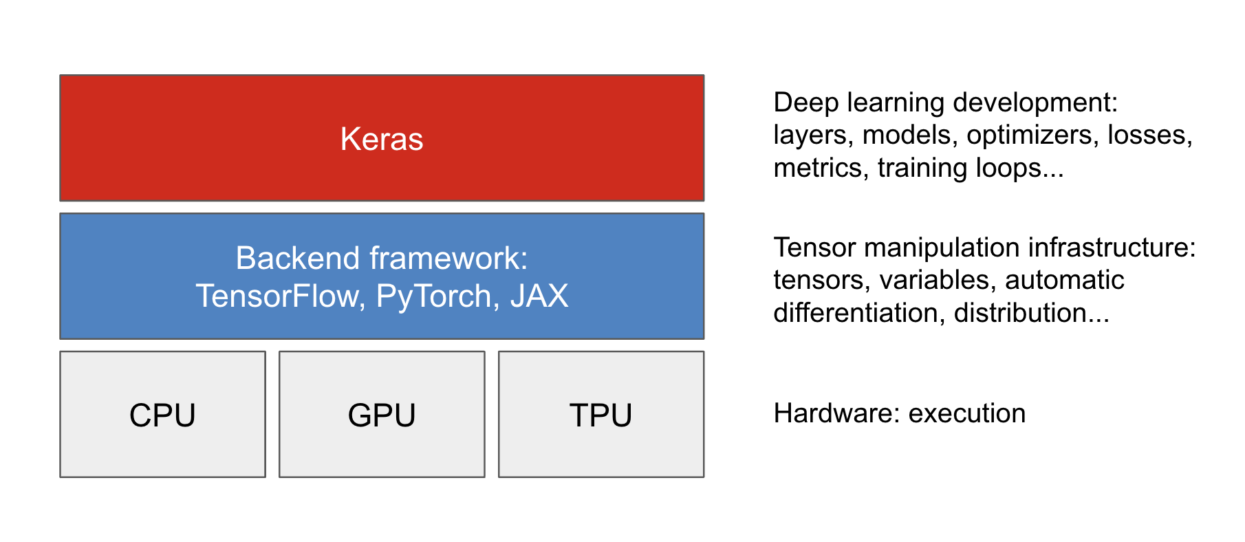
Keras can be used together with JAX, TensorFlow, or PyTorch. They’re the “backend frameworks” of Keras. Through these backend frameworks, Keras can run on top of different types of hardware (see figure 3.4)—GPU, TPU, or plain CPU; it can be seamlessly scaled to thousands of machines, and it can be deployed to a variety of platforms.

Keras and its backends. A backend is a low-level tensor computing platform; Keras is a high-level deep learning API.

Backend frameworks are pluggable: we can switch to a different backend framework after we’ve written Keras code. We aren’t locked into a single framework and a single ecosystem: we can move our models from JAX to TensorFlow to PyTorch depending on our current needs. For instance, when we develop a Keras model, we can debug it with PyTorch, train it on TPU with JAX for maximum efficiency, and finally run inference with the excellent tooling from the TensorFlow ecosystem.

The default backend for Keras right now is TensorFlow, so if you run library(keras3) in a fresh environment without having configured anything, you will be running on top of TensorFlow. There are two ways to pick a different backend:

1. Call the use_backend() function in R. This is the easiest and most convenient approach. Most important, it does more than just inform Keras which backend we need: it also declares all the backend Python dependencies with py_require() so that reticulate can automatically resolve them.

   This means that manually managing a Python installation is not necessary; use_backend() does everything for us!

   library(keras3)
   use_backend("jax")

2. Set the environment variable KERAS_BACKEND, either in a startup file like .Renviron or .Rprofile, or in an R session using Sys.setenv() before the keras3 package is loaded. The R package’s .onLoad() hook automatically reads KERAS_BACKEND and calls use_backend(). As a convenience, we can append a "-cpu" or "-gpu" suffix (for example, KERAS_BACKEND="jax-gpu"). The R package will parse this and call use_backend("jax", gpu = TRUE) to ensure that the correct Python dependencies are declared for GPU- or CPU-only use.

Note

When configuring the Keras backend for PyTorch, use the string "torch" to refer to the PyTorch backend, rather than the string "pytorch", which would be invalid. This is because the PyTorch package name is torch (as in import("torch"), py_require("torch"), or pip install torch).

Now, you may ask, which backend should you choose? It’s really your choice: all the Keras code examples in the rest of the book will be compatible with all three backends. If the need for backend-specific code arises (as in chapter 7, for instance), we will show you all three versions: TensorFlow, PyTorch, and JAX. If you have no particular backend preference, we recommend JAX, with TensorFlow a close second. JAX is usually the most performant backend.

Once your backend is configured, you can start building and training Keras models. Let’s take a look.

3.6.2 Layers: The building blocks of deep learning

The fundamental data structure in neural networks is the layer, to which you were introduced in chapter 2. A layer is a data processing module that takes as input one or more tensors and that outputs one or more tensors. Some layers are stateless, but more frequently layers have a state: the layer’s weights, one or several tensors learned with stochastic gradient descent, which together contain the network’s knowledge.

Different types of layers are appropriate for different tensor formats and different kinds of data processing. For instance, simple vector data, stored in 2D tensors of shape (samples, features), is often processed by densely connected layers, also called fully connected or dense layers (the Dense class in Keras). Sequence data, stored in 3D tensors of shape (samples, timesteps, features), is typically processed by recurrent layers, such as an LSTM layer, or 1D convolution layers (Conv1D). Image data, stored in rank-4 tensors, is usually processed by 2D convolution layers (Conv2D).

You can think of layers as the LEGO bricks of deep learning, a metaphor that is made explicit by Keras. Building deep learning models in Keras is done by clipping together compatible layers to form useful data transformation pipelines.

3.6.2.1 The base Layer class in Keras

A simple API should have a single abstraction around which everything is centered. In Keras, that’s the Layer class. Everything in Keras is either a Layer or something that closely interacts with a Layer.

A Layer is an object that encapsulates some state (weights) and some computation (a forward pass). The weights are typically defined in a build() (although they could also be created in the constructor initialize()), and the computation is defined in the call() method.

In the previous chapter, we implemented a NaiveDense class that contained two weights, W and b, and applied the computation output = activation(matmul(input, W) + b). The following is what the same layer would look like in Keras:

layer_simple_dense <- new_layer_class(
  classname = "SimpleDense",
  initialize = function(units, activation = NULL) {
    super$initialize()
    self$units <- units
    self$activation <- activation
  },
1  build = function(input_shape) {
    .[batch_dim, input_dim] <- input_shape
2    self$W <- self$add_weight(shape(input_dim, self$units),
                              initializer = "random_normal")
    self$b <- self$add_weight(shape(self$units), initializer = "zeros")
  },
3  call = function(inputs) {
    y <- op_matmul(inputs, self$W) + self$b
    if (!is.null(self$activation)) {
      y <- self$activation(y)
    }
    y
  }
)

1

Weight creation takes place in the build() method.

2

add_weight is a shortcut method for creating weights. It’s also possible to create standalone variables and assign them as layer attributes, like: self$W <- keras_variable(shape=..., initializer=...).

3

We define the forward pass computation in the call() method.

In the next section, we’ll cover in detail the purpose of these build() and call() methods. Don’t worry if you don’t understand everything just yet!

Once instantiated, a layer can be used just like a function, taking a tensor as input:

1. Instantiates our layer
2. Creates some test inputs
3. Calls the layer on the inputs, just like a function

my_dense <- layer_simple_dense(units = 32, activation = op_relu)
input_tensor <- op_ones(shape = shape(2, 784))
output_tensor <- my_dense(input_tensor)
op_shape(output_tensor)

shape(2, 32)

1. Instantiates our layer
2. Creates some test inputs
3. Calls the layer on the inputs, just like a function

You’re probably wondering why we had to implement call() and build(), given that we ended up using our layer by calling it. We did that because we want to be able to create the state just in time. Let’s see how that works.

3.6.2.2 Automatic shape inference: Building layers on the fly

Just as with LEGO bricks, you can only “clip” together layers that are compatible. The notion of layer compatibility here refers specifically to the fact that every layer will only accept input tensors of a certain shape and will return output tensors of a certain shape. Consider the following example:

1. A dense layer with 32 output units

1layer <- layer_dense(units = 32, activation = "relu")

1

A dense layer with 32 output units

This layer will return a tensor whose non-batch dimension is 32. It can only be connected to a downstream layer that expects 32-dimensional vectors as its input.

When using Keras, we don’t have to worry about size compatibility most of the time because the layers we add to our models are dynamically built to match the shape of the incoming inputs. For instance, suppose we write the following:

model <- keras_model_sequential() |>
  layer_dense(units = 32, activation = "relu") |>
  layer_dense(units = 32)

The layers don’t receive any information about the shape of their inputs. Instead, they automatically infer their input shape as being the shape of the first inputs they see.

In the toy version of a Dense layer that we implemented in chapter 2, we had to pass the layer’s input size explicitly to the constructor in order to be able to create its weights. That’s not ideal, because it leads to models that look like this, where each new layer needs to be made aware of the shape of the layer before it:

model <- keras_model_sequential() |>
  layer_naive_dense(input_size = 784, output_size = 32, activation = "relu") |>
  layer_naive_dense(input_size = 32, output_size = 64, activation = "relu") |>
  layer_naive_dense(input_size = 64, output_size = 32, activation = "relu") |>
  layer_naive_dense(input_size = 32, output_size = 10, activation = "softmax")

It would be even worse when the rules used by a layer to produce its output shape are complex. For instance, what if our layer returned outputs of shape c(batch, input_size * if (input_size %% 2 == 0) 2 else 3)?

If we were to reimplement our NaiveDense layer as a Keras layer capable of automatic shape inference, it would look like the SimpleDense layer, with its build() and call() methods.

In the Keras SimpleDense, we no longer create weights in the constructor as in the previous example. Instead, we create them in a dedicated state-creation method build(), which receives as an argument the first input shape seen by the layer. The build() method is called automatically the first time the layer is called. In fact, the function that’s actually called when we call a layer is not call() directly, but something that optionally first calls build() before calling call(). The function that’s called when we call a layer schematically looks like this:

`__call__` <- function(inputs) {
  if (!self$built) {
    self$build(op_shape(inputs))
    self$built <- TRUE
  }
  self$call(inputs)
}

With automatic shape inference, our previous example becomes simple and neat:

model <- keras_model_sequential() |>
  layer_simple_dense(units = 32, activation = "relu") |>
  layer_simple_dense(units = 64, activation = "relu") |>
  layer_simple_dense(units = 32, activation = "relu") |>
  layer_simple_dense(units = 10, activation = "softmax")

Note that automatic shape inference is not all the Layer class’ __call__() method handles. It takes care of many more things, in particular routing between eager and graph execution, and input masking (which we cover in chapter 14). For now, just remember: when implementing your own layers, put the forward pass in the call() method.

3.6.3 From layers to models

A deep learning model is a graph of layers. In Keras, that’s the Model class. So far, you’ve only seen Sequential models (a subclass of Model), which are simple stacks of layers, mapping a single input to a single output. But as we move forward, you’ll be exposed to a much wider variety of network topologies. Some common ones are

• Two-branch networks
• Multihead networks
• Residual connections

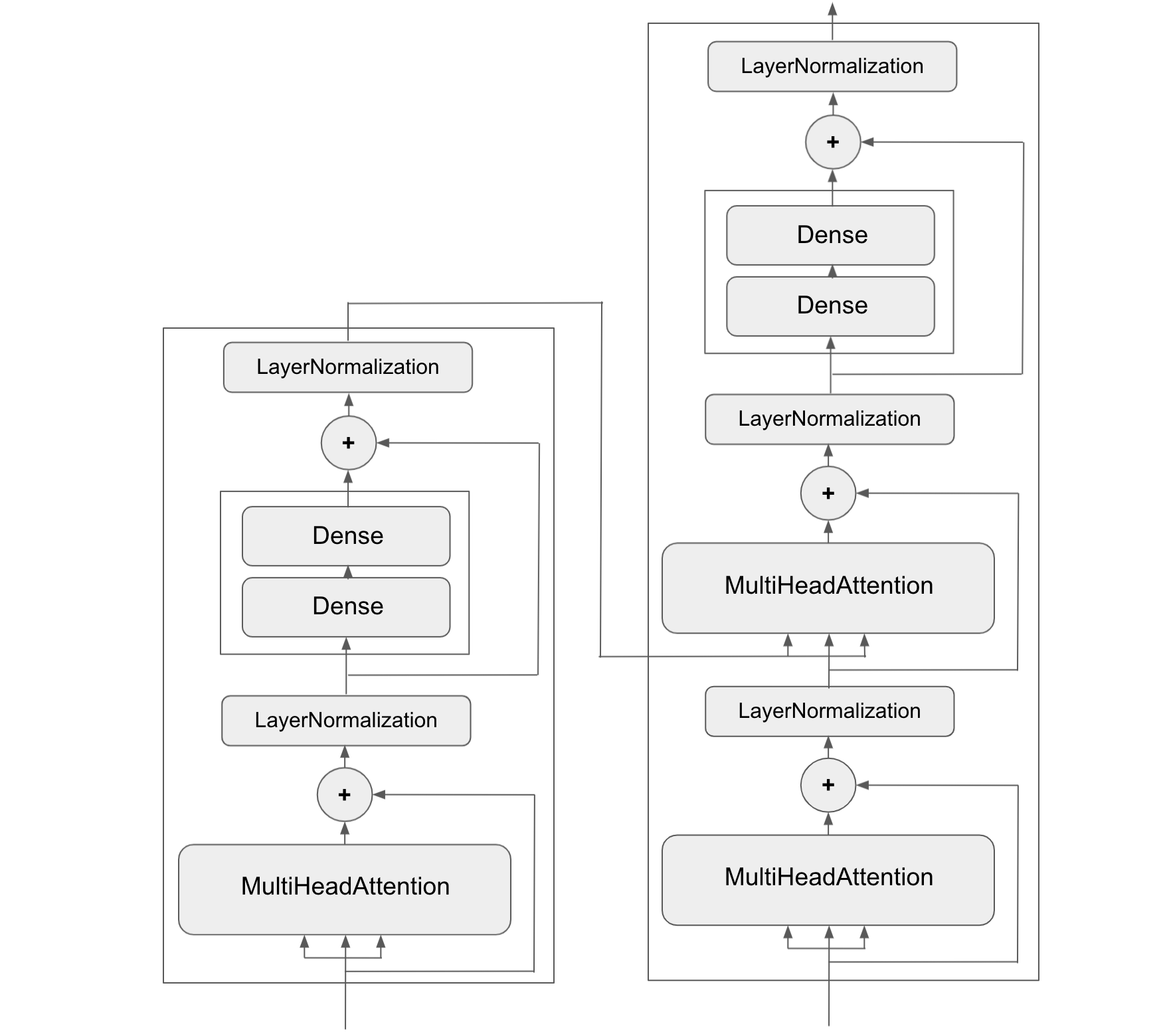
Network topology can get involved. For instance, figure 3.5 shows the topology of the graph of layers of a Transformer, a common architecture designed to process text data.

The Transformer architecture. There’s a lot going on here. Throughout the coming chapters, we’ll build up the concepts you need, and by the end of chapter 15 you’ll understand it.

There are generally two ways to build such models in Keras: directly subclass the Model class, or use the Functional API, which lets us do more with less code. We’ll cover both approaches in chapter 7.

The topology of a model defines a hypothesis space. You may remember that in chapter 1, we described machine learning as “searching for useful representations of some input data, within a predefined space of possibilities, using guidance from a feedback signal.” By choosing a network topology, we constrain our space of possibilities (hypothesis space) to a specific series of tensor operations, mapping input data to output data. What we’ll then be searching for is a good set of values for the weight tensors involved in these tensor operations.

To learn from data, we have to make assumptions about it. These assumptions define what can be learned. As such, the structure of our hypothesis space— the architecture of our model—is extremely important. It encodes the assumptions we make about our problem: the prior knowledge that the model starts with. For instance, if we’re working on a two-class classification problem with a model made of a single Dense layer with no activation (a pure affine transformation), we are assuming that our two classes are linearly separable.

Picking the right network architecture is more of an art than a science, and although there are some best practices and principles you can rely on, only practice can help you become a proper neural network architect. The next few chapters will both teach you explicit principles for building neural networks and help you develop intuition as to what works or doesn’t work for specific problems. You’ll build a solid intuition about what type of model architectures work for different kinds of problems, how to build these networks in practice, how to pick the right learning configuration, and how to tweak a model until it yields the results you want to see.

3.6.4 The “compile” step: Configuring the learning process

Once the model architecture is defined, we still have to choose three more things:

• Loss function (objective function)  – The quantity that will be minimized during training. It represents a measure of success for the task at hand.

• Optimizer  – Determines how the network will be updated based on the loss function. It implements a specific variant of stochastic gradient descent (SGD).

• Metrics – The measures of success you want to monitor during training and validation, such as classification accuracy. Unlike the loss, training will not optimize directly for these metrics. As such, metrics don’t need to be differentiable.

Once we’ve picked our loss, optimizer, and metrics, we can use the built-in compile() and fit() methods to start training our model. Alternatively, we can write our own custom training loops; we cover how to do this in chapter 7. It’s a lot more work! For now, let’s take a look at compile() and fit().

The compile() method configures the training process; you were introduced to it in our very first neural network example in chapter 2. It takes the arguments optimizer, loss, and metrics (which can be a list):

1model <- keras_model_sequential() |> layer_dense(units = 1)
model |> compile(
2  optimizer = "rmsprop",
3  loss = "mean_squared_error",
4  metrics = c("accuracy")
)

1

Defines a linear classifier

2

Specifies the optimizer by name: RMSprop (it’s case-insensitive)

3

Specifies the loss by name: mean squared error

4

Specifies a list of metrics: in this case, only accuracy

In the previous call to compile(), we passed the optimizer, loss, and metrics as strings (such as "rmsprop"). These strings are actually shortcuts that get converted to Keras objects. For instance, "rmsprop" becomes optimizer_rmsprop(). Importantly, it’s also possible to specify these arguments as object instances, like this:

model |> compile(
  optimizer = optimizer_rmsprop(),
  loss = loss_mean_squared_error(),
  metrics = list(metric_binary_accuracy())
)

This is useful if we want to pass our own custom losses or metrics, or if we want to further configure the objects we’re using—for instance, by passing a learning_rate argument to the optimizer:

model |> compile(
  optimizer = optimizer_rmsprop(learning_rate = 1e-4),
  loss = my_custom_loss,
  metrics = c(my_custom_metric_1, my_custom_metric_2)
)

In chapter 7, we cover how to create custom losses and metrics. In general, you won’t have to create your own losses, metrics, or optimizers from scratch because Keras offers a wide range of built-in options that are likely to include what you need:

• Optimizers

  • optimizer_sgd() (with or without momentum)
  • optimizer_rmsprop()
  • optimizer_adam()
  • Etc.

• Losses

  • loss_categorical_crossentropy()
  • loss_sparse_categorical_crossentropy()
  • loss_binary_crossentropy()
  • loss_mean_squared_error()
  • loss_kl_divergence()
  • loss_cosine_similarity()
  • Etc.

• Metrics

  • metric_categorical_accuracy()
  • metric_sparse_categorical_accuracy()
  • metric_binary_accuracy()
  • metric_auc()
  • metric_precision()
  • metric_recall()
  • Etc.

Throughout this book, you’ll see concrete applications of many of these options.

3.6.5 Picking a loss function

Choosing the right loss function for the right problem is extremely important: our network will take any shortcut it can to minimize the loss. So, if the objective doesn’t fully correlate with success for the task at hand, our network will end up doing things we may not have wanted. Imagine a stupid, omnipotent AI trained via SGD, with this poorly chosen objective function: “Maximize the average well-being of all humans alive.” To make its job easier, this AI might choose to kill all humans except a few and focus on the well-being of the remaining ones because average well-being isn’t affected by how many humans are left. That might not be what we intended! Just remember that all neural networks you build will be just as ruthless in lowering their loss function, so choose the objective wisely, or you’ll have to face unintended side effects.

Fortunately, when it comes to common problems such as classification, regression, and sequence prediction, there are simple guidelines you can follow to choose the correct loss. For instance, you’ll use binary cross-entropy for a two-class classification problem, categorical cross-entropy for a many-class classification problem, and so on. Only when you’re working on truly new research problems will you have to develop your own loss functions. In the next few chapters, we’ll detail explicitly which loss functions to choose for a wide range of common tasks.

3.6.6 Understanding the fit() method

After compile() comes fit(). The fit method implements the training loop. Its key arguments are as follows:

• The data (inputs and targets) to train on. It will typically be passed either in the form of R or NumPy arrays or a TensorFlow Dataset object. You’ll learn more about the Dataset API in the upcoming chapters.
• The number of epochs to train for: how many times the training loop should iterate over the data passed.
• The batch size to use within each epoch of mini-batch gradient descent: the number of training examples considered to compute the gradients for one weight update step.

Here’s what it looks like to fit a model for five epochs:

history <- model |> fit(
1  inputs,
2  targets,
3  epochs = 5,
4  batch_size = 128
)

1

The input examples, as an R array

2

The corresponding training targets, as an R array

3

The training loop will iterate over the data five times.

4

The training loop will iterate over the data in batches of 128 examples.

The call to fit() returns a keras_training_history object. This object contains metrics, which is a named list of their per-epoch values for "loss" and specific metric names:

str(history$metrics)

List of 2
 $ binary_accuracy: num [1:5] 0.039 0.041 0.043 0.044 0.0445
 $ loss           : num [1:5] 7.89 7.55 7.27 7.01 6.74

A history object can also be converted to a data frame:

tibble::as_tibble(history)

# A tibble: 10 × 4
   epoch  value metric          data    
   <int>  <dbl> <fct>           <fct>   
 1     1 0.0390 binary_accuracy training
 2     2 0.0410 binary_accuracy training
 3     3 0.0430 binary_accuracy training
 4     4 0.0440 binary_accuracy training
 5     5 0.0445 binary_accuracy training
 6     1 7.89   loss            training
 7     2 7.55   loss            training
 8     3 7.27   loss            training
 9     4 7.01   loss            training
10     5 6.74   loss            training

3.6.7 Monitoring loss and metrics on validation data

The goal of machine learning is not to obtain models that perform well on the training data, which is easy: all we have to do is follow the gradient. The goal is to obtain models that perform well in general, particularly on data points that the model has never encountered before. Just because a model performs well on its training data doesn’t mean it will perform well on data it has never seen before! For instance, it’s possible that our model could end up merely memorizing a mapping between our training samples and their targets, which would be useless for the task of predicting targets for data the model has never seen before. We’ll go over this point in much more detail in chapter 5.

To keep an eye on how the model does on new data, it’s standard practice to reserve a subset of the training data as validation data: we won’t train the model on this data, but we will use it to compute a loss value and a metrics value. We do this by using the validation_data argument in fit(). Like the training data, the validation data can be passed as R or NumPy arrays or as a TensorFlow Dataset object:

model <- keras_model_sequential() |> layer_dense(units = 1)

model |> compile(
  optimizer = optimizer_rmsprop(learning_rate = 0.1),
  loss = loss_mean_squared_error(),
  metrics = list(metric_binary_accuracy())
)

1indices_permutation <- sample.int(nrow(inputs))
shuffled_inputs <- inputs[indices_permutation, , drop = FALSE]
shuffled_targets <- targets[indices_permutation, , drop = FALSE]

2num_validation_samples <- as.integer(0.3 * nrow(inputs))
val_inputs <- shuffled_inputs[1:num_validation_samples, ]
val_targets <- shuffled_targets[1:num_validation_samples, ]
training_inputs <- shuffled_inputs[-(1:num_validation_samples), ]
training_targets <- shuffled_targets[-(1:num_validation_samples), ]

model |> fit(
3  training_inputs, training_targets,
  epochs = 5, batch_size = 16,
4  validation_data = list(val_inputs, val_targets)
)

1

Shuffles the inputs and targets using a random index permutation, to avoid having samples from only one class in the validation data

2

Reserves 30% of the training inputs and targets for validation (we’ll exclude these samples from training and reserve them to compute the validation loss and metrics)

3

Training data, used to update the weights of the model

4

Validation data, used only to monitor the validation loss and metrics

The value of the loss on the validation data is called the validation loss, to distinguish it from the training loss. Note that it’s essential to keep the training data and validation data strictly separate: the purpose of validation is to monitor whether what the model is learning is actually useful on new data. If any of the validation data has been seen by the model during training, our validation loss and metrics will be flawed.

If we want to compute the validation loss and metrics after training is complete, we can call the evaluate() method:

loss_and_metrics <- evaluate(model, val_inputs, val_targets, batch_size = 128)

evaluate() will iterate in batches (of size batch_size) over the data passed and return a list of scalars, where the first entry is the validation loss and the following entries are the validation metrics. If the model has no metrics, only the validation loss is returned (rather than a list).

3.6.8 Inference: Using a model after training

Once we’ve trained our model, we can use it to make predictions on new data. This is called inference. To do this, a naive approach would simply be to call the model:

1predictions <- model(new_inputs)

1

Takes an array or a tensor for our current backend and returns a tensor for our current backend

However, this will process all inputs in new_inputs at once, which may not be feasible if we’re looking at a lot of data (in particular, it may require more memory than our GPU has).

A better way to do inference is to use the predict() method. It will iterate over the data in small batches and return an R array of predictions. And unlike the previous method, it can also process TensorFlow Dataset objects:

1predictions <- predict(model, new_inputs, batch_size = 128)

1

Takes an R or NumPy array or a TensorFlow Dataset and returns an R array

For instance, if we use predict() on some of our validation data with the linear model we trained earlier, we get scalar scores that correspond to the model’s prediction for each input sample:

predictions <- model |> predict(val_inputs, batch_size = 128)
head(predictions)

           [,1]
[1,] 0.77219641
[2,] 0.95900345
[3,] 0.17848289
[4,] 0.01958176
[5,] 0.67687637
[6,] 0.80361819

For now, this is all you need to know about Keras models. You are ready to move on to solving real-world machine problems with Keras in the next chapter.

3.7 Summary

• TensorFlow, PyTorch, and JAX are three popular low-level frameworks for numerical computation and automatic differentiation. They all have their own way of doing things and their own strengths and weaknesses.
• Keras is a high-level API for building and training neural networks. It can be used with TensorFlow, PyTorch, or JAX—just pick the backend you like best.
• The central class of Keras is the Layer. A layer encapsulates some weights and some computation. Layers are assembled into models.
• Before you start training a model, you need to pick an optimizer, a loss, and some metrics, which you specify via the compile() method.
• To train a model, you can use the fit() method, which runs mini-batch gradient descent for you. You can also use it to monitor your loss and metrics on validation data, a set of inputs that the model doesn’t see during training.
• Once your model is trained, you can use the predict() method to generate predictions on new inputs.

---

1. R. E. Wengert, “A Simple Automatic Derivative Evaluation Program,” Communications of the ACM, 7 no. 8 [1964].