12 Object detection

This chapter covers

Understanding the object detection problem
Two-stage and single-stage object detectors
Training a simple single-stage detector from scratch
Using a pretrained object detector

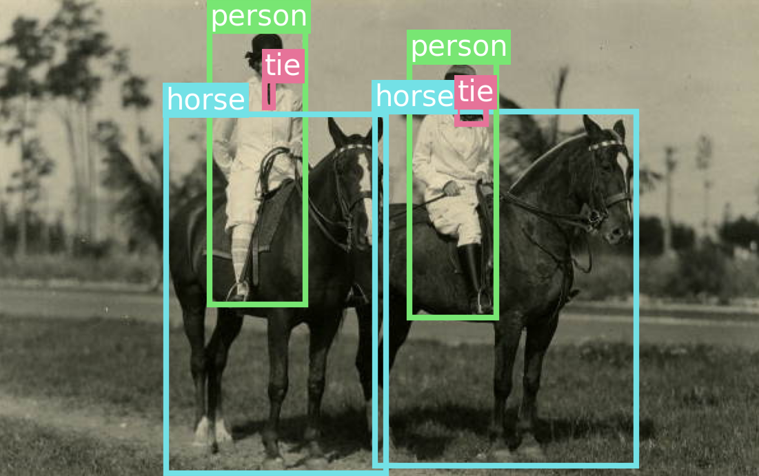
Object detection is all about drawing boxes (called bounding boxes) around objects of interest in a picture (see figure 12.1). This enables us to know not just which objects are in a picture but also where they are. Some of its most common applications are as follows:

Counting—Find out how many instances of an object are in an image.
Tracking—Track how objects move in a scene over time by performing object detection on every frame of a movie.
Cropping—Identify the area of an image that contains an object of interest to crop it and send a higher-resolution version of the image patch to a classifier or an optical character recognition (OCR) model.

Object detectors draw boxes around objects in an image and label them.

You might be thinking, if I have a segmentation mask for an object instance, I can already compute the coordinates of the smallest box that contains the mask. So couldn’t we just use image segmentation all the time? Do we need object detection models at all?

Indeed, segmentation is a strict superset of detection. It returns all the information that could be returned by a detection model—and then a lot more. This increased wealth of information has a significant computational cost: a good object detection model will typically run much faster than an image segmentation model. It also has a data labeling cost: to train a segmentation model, we need to collect pixel-precise masks, which are much more time-consuming to produce than the mere bounding boxes required by object detection models. As a result, you will always want to use an object detection model if you have no need for pixel-level information—for instance, if all you want is to count objects in an image.

12.1 Single-stage vs. two-stage object detectors

There are two broad categories of object detection architectures:

Two-stage detectors, which first extract region proposals, known as region-based convolutional neural network (R-CNN) models
Single-stage detectors, such as RetinaNet and the You Only Look Once family of models

Here’s how they work.

12.1.1 Two-stage R-CNN detectors

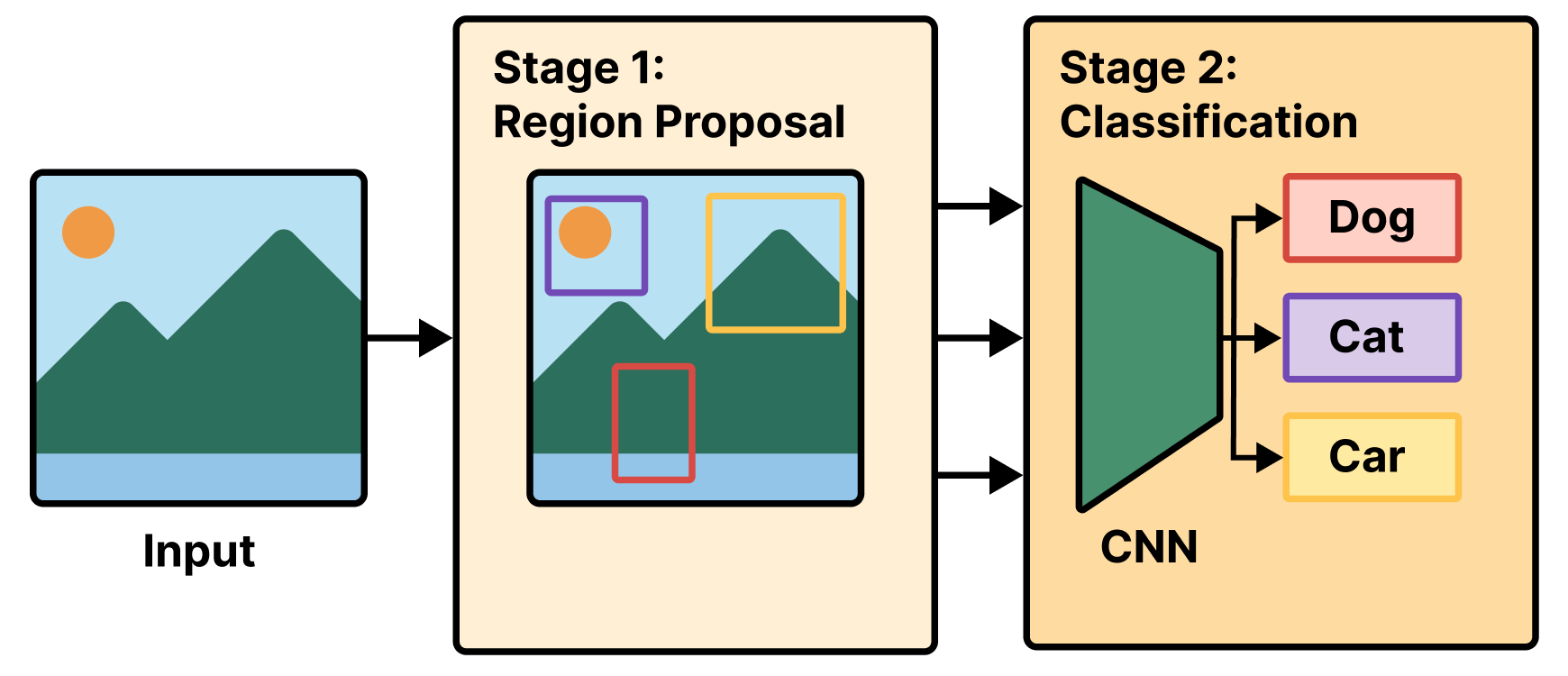
A region-based convnet, or R-CNN model, is a two-stage model. The first stage takes an image and produces a few thousand partially overlapping bounding boxes around areas that look object-like. These boxes are called region proposals. This stage isn’t very smart, so at that point we aren’t sure whether the proposed regions do contain objects and, if so, what objects they contain.

That’s the job of the second stage: a convnet that looks at each region proposal and classifies it into a number of predetermined classes, just like the models you saw in chapter 9 (see figure 12.2). Region proposals that have a low score across all classes considered are discarded. We are then left with a much smaller set of boxes, each with a high class presence score for one particular class. Finally, bounding boxes around each object are further refined to eliminate duplicates and make each bounding box as precise as possible.

An R-CNN first extracts region proposals and then classifies the proposals with a convnet (a CNN).

In early R-CNN versions, the first stage was a heuristic model called Selective Search that used some definition of spatial consistency to identify object-like areas. Heuristic is a term you’ll hear quite a lot in machine learning—it simply means “a bundle of hard-coded rules someone made up.” It’s usually used in opposition to learned models (where the rules are automatically derived) or theory-derived models. In later versions of R-CNN, such as faster-R-CNN, the box-generation stage became a deep learning model called a region proposal network.

The two-stage approach of R-CNN works very well in practice, but it’s computationally expensive, most notably because it requires us to classify thousands of patches for every single image we process. That makes it unsuitable for most real-time applications and for embedded systems. Our take is that in practical applications, we generally don’t need a computationally expensive object detection system like R-CNN: if we’re doing server-side inference with a beefy GPU, we’ll probably be better off using a segmentation model instead, like the Segment Anything model you saw in the previous chapter. And if we’re resource-constrained, we’re going to want to use a more computationally efficient object detection architecture—a single-stage detector.

12.1.2 Single-stage detectors

Around 2015, researchers and practitioners began experimenting with using a single deep learning model to jointly predict bounding box coordinates together with their labels, an architecture called a single-stage detector. The main families of single-stage detectors are RetinaNet, single-shot multibox detectors (SSDs), and the You Only Look Once family (YOLO). Yes, like the meme. That’s on purpose.

Single-stage detectors, especially recent YOLO iterations, boast significantly faster speeds and greater efficiency than their two-stage counterparts, albeit with a minor potential tradeoff in accuracy. Nowadays, YOLO is arguably the most popular object detection model out there, especially when it comes to real-time applications. A new version usually comes out every year—interestingly, each new version tends to be developed by a separate organization.

In the next section, we will build a simplified YOLO model from scratch.

12.2 Training a YOLO model from scratch

View on GitHub Run on Colab

Overall, building an object detector can be an undertaking—not that there’s anything theoretically complex about it. We just need a lot of code to handle manipulating bounding boxes and predicted output. To keep things simple, we will re-create the very first YOLO model from 2015. There are 12 YOLO versions as of this writing, but the original is a bit simpler to work with.

12.2.1 Downloading the COCO dataset

Before we start creating our model, we need data to train with. The COCO dataset (https://cocodataset.org/; most images in this chapter are from this dataset), short for Common Objects in Context, is one of the best-known and most commonly used object detection datasets. It consists of real-world photos from a number of different sources, plus human-created annotations. These include object labels, bounding box annotations, and full segmentation masks. We will disregard the segmentation masks and just use bounding boxes.

Let’s download the 2017 version of the COCO dataset. Although it isn’t large by today’s standards, this 18 GB dataset will be the largest dataset we use in the book. If you are running the code as you read, this is a good chance to take a breather.

Listing 12.1: Downloading the 2017 COCO dataset

library(keras3)
py_require("keras-hub")
keras_hub <- import("keras_hub")

images_path <- get_file(
  "coco",
  "http://images.cocodataset.org/zips/train2017.zip",
  extract = TRUE
)

annotations_path <- get_file(
  "annotations",
  "http://images.cocodataset.org/annotations/annotations_trainval2017.zip",
  extract = TRUE
)

We need to do some input massaging before we are ready to use this data. The first download gives us an unlabeled directory of all the COCO images, and the second download includes all the image metadata via a JSON file. COCO associates each image file with an ID, and each bounding box is paired with one of these IDs. We need to collate all the box and image data together.

Each bounding box comes with (x, y, width, height) pixel coordinates starting at the top-left corner of the image. As we load our data, we can rescale all bounding box coordinates so they are points in a [0, 1] unit square. This will make it easier to manipulate these boxes without needing to check the size of each input image.

Listing 12.2: Parsing the COCO data

library(dplyr, warn.conflicts = FALSE)

raw_annotations <-
  fs::path(annotations_path, "annotations/instances_train2017.json") |>
  yyjsonr::read_json_file() |>
  lapply(\(x) if (is.data.frame(x)) as_tibble(x) else x)

1images <- raw_annotations$images |>
  select(file_name, height, width, image_id = id)

annotations <- raw_annotations$annotations |>
2  summarise(
    .by = image_id,
    labels = list(category_id),
    boxes = list({
      boxes <- matrix(unlist(bbox), byrow = TRUE, ncol = 4)
      colnames(boxes) <- c("left", "top", "width", "height")
      boxes
    })
  )

3scale_boxes <- function(boxes, height, width) {
4  if (width > height) {
    boxes[, "top"] <- boxes[, "top"] + (width - height) / 2
    scale <- width
  } else if (height > width) {
    boxes[, "left"] <- boxes[, "left"] + (height - width) / 2
    scale <- height
  } else {
    scale <- width
  }

  boxes / scale
}

metadata <-
  inner_join(annotations, images, by = "image_id") |>
  mutate(
    boxes = Map(scale_boxes, boxes, height, width),
    labels,
    path = fs::path(images_path, "train2017", file_name),
    .keep = "none"
  )

5rm(raw_annotations, annotations, images)

1: Image metadata is one row per image.
2: Summarizes annotations to also be one row per image
3: Function to convert bounding box coordinates to a unit square [0, 1]
4: Pads the shorter side to make the image square and centered before scaling
5: Frees memory: we’ll only need metadata going forward.

Let’s take a look at the data we just loaded.

Listing 12.3: Inspecting the COCO data

metadata

# A tibble: 117,266 × 3
  labels     boxes          path                                            
  <list>     <list>         <fs::path>                                      
1 <int [11]> <dbl [11 × 4]> ….keras/datasets/coco/train2017/000000558840.jpg
2 <int [9]>  <dbl [9 × 4]>  ….keras/datasets/coco/train2017/000000200365.jpg
3 <int [19]> <dbl [19 × 4]> ….keras/datasets/coco/train2017/000000495357.jpg
4 <int [22]> <dbl [22 × 4]> ….keras/datasets/coco/train2017/000000116061.jpg
5 <int [2]>  <dbl [2 × 4]>  ….keras/datasets/coco/train2017/000000016164.jpg
# ℹ 117,261 more rows

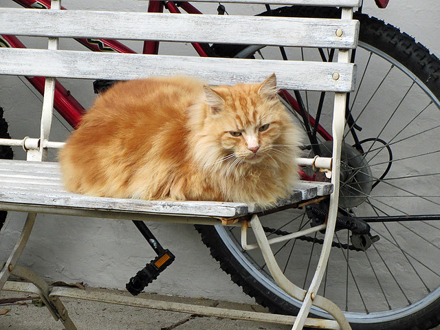
range(sapply(metadata$boxes, nrow))

[1]  1 93

max(unlist(metadata$labels))

[1] 90

We have 117,266 images. Each image can include anywhere from 1 to 93 objects with an associated bounding box. There are only 91 possible labels for objects, chosen by the COCO dataset creators.

We can use a KerasHub utility keras_hub$utils$coco_id_to_name(id) to map these integer labels to human-readable names, similar to the utility we used to decode ImageNet predictions to text labels back in chapter 8.

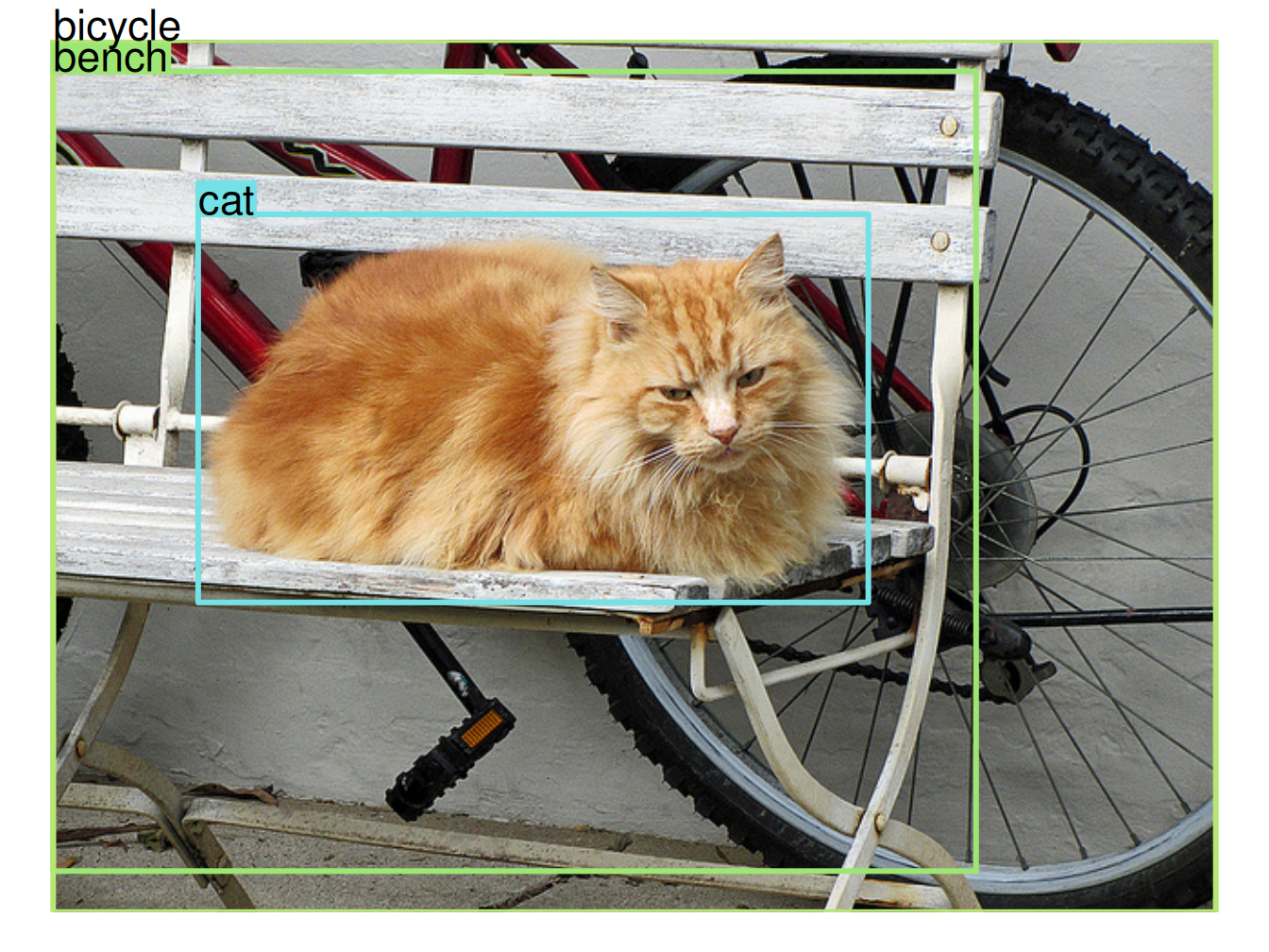
example <- metadata[436, ] |> lapply(`[[`, 1)
example$labels |> sapply(keras_hub$utils$coco_id_to_name)

[1] "cat"     "bench"   "bicycle"

Let’s visualize an example image to make this a little more concrete. We can define a function to draw an image and another function to draw a labeled bounding box on this image. We will need both of these throughout the chapter. We can use the HSV colorspace as a simple trick to generate new colors for each new label we see. By fixing the saturation and brightness of the color and only updating its hue, we can generate bright new colors that stand out clearly from our image.

Listing 12.4: Visualizing a COCO image with box annotations

label_to_color <- function(label, alpha = 1) {
  ifelse(label == 0, "gray", hsv(
1    h = (label * 0.618) %% 1,
    s = 0.5,
    v = 0.9,
    alpha = alpha
  ))
}

2draw_image <- function(image_path, show_padding = FALSE) {
  img <- jpeg::readJPEG(image_path, native = TRUE)
  par(mar = rep(1.1, 4), xaxs = "i", yaxs = "i")
  plot.new()
3  if (nrow(img) > ncol(img)) {
    x_pad <- (nrow(img) - ncol(img)) / nrow(img) / 2
    plot.window(
      xlim = if (show_padding) 0:1 else c(x_pad, 1 - x_pad),
      ylim = 0:1,
      asp = 1
    )
    rasterImage(img, x_pad, 0, 1 - x_pad, 1)
  } else if (ncol(img) > nrow(img)) {
    y_pad <- (ncol(img) - nrow(img)) / ncol(img) / 2
    plot.window(
      xlim = 0:1,
      ylim = if (show_padding) 0:1 else c(y_pad, 1 - y_pad),
      asp = 1
    )
    rasterImage(img, 0, y_pad, 1, 1 - y_pad)
  } else {
    plot.window(0:1, 0:1, asp = 1)
    rasterImage(img, 0, 0, 1, 1)
  }
}

draw_boxes <- function(boxes, text, color) {
  boxes <- as.data.frame(as.matrix(boxes))
  stopifnot(c("left", "top", "width", "height") %in% names(boxes))
4  rect(
    xleft = boxes$left, xright = boxes$left + boxes$width,
    ytop = 1 - boxes$top, ybottom = 1 - boxes$top - boxes$height,
    border = color, lwd = 3
  )
5  rect(
    xleft = boxes$left, xright = boxes$left + strwidth(text, cex = 1.4),
    ytop = 1 - boxes$top + strheight(text, cex = 1.4), ybottom = 1 - boxes$top,
    col = color, border = color, lwd = 3
  )
6  text(boxes$left, 1 - boxes$top, text,
       adj = c(0, 0), col = "black", cex = 1.4, xpd = NA)
}

1: Uses the golden ratio to generate new hues of a bright color with the HSV colorspace
2: draw_image() is almost identical to plot(as.raster()), except it sets up the plotting region to be [0, 1]; these are more convenient coordinates for drawing our scaled box annotations.
3: Centers the image in the unit square
4: Draws the bounding boxes
5: Draws a colored underlay for text labels
6: Draws the text labels

Let’s use our new visualization to look at our sample image (see figure 12.3):

example <- metadata[436, ] |> lapply(`[[`, 1)
draw_image(example$path)
draw_boxes(
  boxes = example$boxes,
  text =  example$labels |> sapply(keras_hub$utils$coco_id_to_name),
  color = example$labels |> label_to_color()
)

YOLO outputs a bounding box prediction and class label for each image region.¹

Although it would be fun to train on all 18 GB of our input data, we want to keep the examples in this book easily runnable on modest hardware. If we limit ourselves to only images with four or fewer boxes, we will make our training problem easier and halve the data size. Let’s do this and shuffle our data—the images are grouped by object type, which would be terrible for training:

metadata <- metadata |>
  filter(lengths(labels) <= 4) |>
  slice(sample.int(n()))

That’s it for data loading! Let’s start creating our YOLO model.

12.2.2 Creating a YOLO model

As mentioned previously, the YOLO model is a single-stage detector. Rather than first identifying all candidate objects in a scene and then classifying the object regions, YOLO proposes bounding boxes and object labels in a single step.

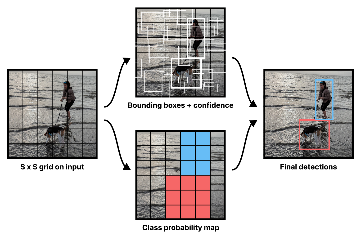
Our model will divide an image into a grid and predict two separate outputs at each grid location: a bounding box and a class label. In the original paper by Joseph Redmon et al.², the model predicted multiple boxes per grid location, but we’ll keep things simple and just predict one box in each grid square.

Most images do not have objects evenly distributed across a grid, and to account for this, the model will output a confidence score along with each box, as shown in figure 12.4. We’d like this confidence to be high when an object is detected at a location and zero when there’s no object. Most grid locations will have no object and should report a near-zero confidence.

YOLO outputs as visualized in the first YOLO paper

Like many models in computer vision, the YOLO model uses a convnet backbone to obtain interesting high-level features for an input image, a concept we first explored in chapter 8. In their paper, Redmon et al. created their own backbone model and pretrained it with ImageNet for classification. Rather than do this ourselves, we can instead use KerasHub to load a pretrained backbone.

Instead of using the Xception backbone we’ve used so far in this book, we will switch to ResNet, a family of models we first mentioned in chapter 9. The structure is similar to Xception, but ResNet uses strides instead of pooling layers to downsample the image. As we mentioned in chapter 11, strided convolutions are better when we care about the spatial location of the input.

Let’s load up our pretrained model and matching preprocessing (to rescale the image). We will resize our images to 448 × 448; image input size is important for the object detection task.

Listing 12.5: Loading the ResNet model

image_size <- c(448, 448)

backbone <- keras_hub$models$Backbone$from_preset(
  "resnet_50_imagenet"
)
preprocessor <- keras_hub$layers$ImageConverter$from_preset(
  "resnet_50_imagenet",
  image_size = shape(image_size)
)

Next, we can turn our backbone into a detection model by adding new layers for outputting box and class predictions. The setup proposed in the YOLO paper is simple. Take the output of a convnet backbone, and feed it through two densely connected layers with an activation in the middle. Then split the output. The first five numbers will be used for bounding box prediction (four for the box and one for the box confidence). The rest will be used for the class probability map shown in figure 12.4—a classification prediction for each grid location over all possible 91 labels.

Let’s write this out.

Listing 12.6: Attaching a YOLO prediction head

grid_size <- 6L
num_labels <- 91L

inputs <- keras_input(shape = c(image_size, 3))
x <- inputs |>
  backbone() |>
1  layer_conv_2d(512, c(3, 3), strides = c(2, 2)) |>
  layer_flatten() |>
  layer_dense(2048, activation = "relu",
2              kernel_initializer = "glorot_normal") |>
  layer_dropout(0.5) |>
  layer_dense(grid_size * grid_size * (num_labels + 5)) |>
3  layer_reshape(c(grid_size, grid_size, num_labels + 5))

4box_predictions <- x@r[.., 1:5]
class_predictions <- layer_activation_softmax(x@r[.., 6:NA])
outputs <- list(box = box_predictions, class = class_predictions)
model <- keras_model(inputs, outputs)

1: Makes the backbone outputs smaller and then flattens the output features
2: Passes the flattened feature maps through two densely connected layers
3: Reshapes outputs to a 6 by 6 grid
4: Splits box and class predictions

We can get a better sense of the model by looking at the model summary:

model

Model: "functional"
┏━━━━━━━━━━━━━━━━━━━┳━━━━━━━━━━━━━━━━━┳━━━━━━━━━━━┳━━━━━━━━━━━━━━━━┳━━━━━━━┓
┃ Layer (type)      ┃ Output Shape    ┃   Param # ┃ Connected to   ┃ Trai… ┃
┡━━━━━━━━━━━━━━━━━━━╇━━━━━━━━━━━━━━━━━╇━━━━━━━━━━━╇━━━━━━━━━━━━━━━━╇━━━━━━━┩
│ input_layer_1     │ (None, 448,     │         0 │ -              │   -   │
│ (InputLayer)      │ 448, 3)         │           │                │       │
├───────────────────┼─────────────────┼───────────┼────────────────┼───────┤
│ res_net_backbone  │ (None, 14, 14,  │ 23,561,1… │ input_layer_1… │   Y   │
│ (ResNetBackbone)  │ 2048)           │           │                │       │
├───────────────────┼─────────────────┼───────────┼────────────────┼───────┤
│ conv2d (Conv2D)   │ (None, 6, 6,    │ 9,437,696 │ res_net_backb… │   Y   │
│                   │ 512)            │           │                │       │
├───────────────────┼─────────────────┼───────────┼────────────────┼───────┤
│ flatten (Flatten) │ (None, 18432)   │         0 │ conv2d[0][0]   │   -   │
├───────────────────┼─────────────────┼───────────┼────────────────┼───────┤
│ dense (Dense)     │ (None, 2048)    │ 37,750,7… │ flatten[0][0]  │   Y   │
├───────────────────┼─────────────────┼───────────┼────────────────┼───────┤
│ dropout (Dropout) │ (None, 2048)    │         0 │ dense[0][0]    │   -   │
├───────────────────┼─────────────────┼───────────┼────────────────┼───────┤
│ dense_1 (Dense)   │ (None, 3456)    │ 7,081,344 │ dropout[0][0]  │   Y   │
├───────────────────┼─────────────────┼───────────┼────────────────┼───────┤
│ reshape (Reshape) │ (None, 6, 6,    │         0 │ dense_1[0][0]  │   -   │
│                   │ 96)             │           │                │       │
├───────────────────┼─────────────────┼───────────┼────────────────┼───────┤
│ get_item_1        │ (None, 6, 6,    │         0 │ reshape[0][0]  │   -   │
│ (GetItem)         │ 91)             │           │                │       │
├───────────────────┼─────────────────┼───────────┼────────────────┼───────┤
│ get_item          │ (None, 6, 6, 5) │         0 │ reshape[0][0]  │   -   │
│ (GetItem)         │                 │           │                │       │
├───────────────────┼─────────────────┼───────────┼────────────────┼───────┤
│ softmax (Softmax) │ (None, 6, 6,    │         0 │ get_item_1[0]… │   -   │
│                   │ 91)             │           │                │       │
└───────────────────┴─────────────────┴───────────┴────────────────┴───────┘
 Total params: 77,830,976 (296.90 MB)
 Trainable params: 77,777,856 (296.70 MB)
 Non-trainable params: 53,120 (207.50 KB)

Our backbone outputs have shape (batch_size, 14, 14, 2048). That is 401,408 output floats per image, a bit too many to feed into our dense layers. We downscale the feature maps with a strided conv layer to (batch_size, 6, 6, 512) with a more manageable 18,432 floats per image.

Next, we can add our two densely connected layers. We flatten the entire feature map, pass it through a Dense layer with a relu activation, and then pass it through a final Dense layer with our exact number of output predictions: 5 for the bounding box and confidence and 91 for each object class at each grid location.

Finally, we reshape the outputs back to a 6 × 6 grid and split our box and class predictions. As usual for our classification outputs, we apply a softmax. The box outputs will need more special consideration; we will cover this later.

Looking good! Note that because we flatten the entire feature map through the classification layer, every grid detector can use the entire image’s features; there’s no locality constraint. This is by design: large objects will not stay contained to a single grid cell.

12.2.3 Readying the COCO data for the YOLO model

Our model is relatively simple, but we still need to preprocess our inputs to align them with the prediction grid. Each grid detector will be responsible for detecting any boxes whose center falls inside the grid box. Our model will output five floats for the box (x, y, w, h, confidence). The x and y will represent the object’s center relative to the bounds of the grid cell (from 0 to 1). The w and h will represent the object’s size relative to the image size.

We already have the right w and h values in our training data. However, we need to translate our x and y values to and from the grid. Let’s define two utilities:

to_grid <- function(box) {
  .[x, y, w, h] <- box
  .[cx, cy] <- c(x + w / 2, y + h / 2) * grid_size
  .[ix, iy] <- as.integer(c(cx, cy))
  grid_box <- c(cx - ix, cy - iy, w, h)
  list(cell = c(ix, iy), box = grid_box)
}

from_grid <- function(cell, box) {
  .[xi, yi] <- cell
  .[x, y, w, h] <- box
  x <- (xi + x) / grid_size - w / 2
  y <- (yi + y) / grid_size - h / 2
  cbind(left = x, top = y, width = w, height = h)
}

Let’s rework our training data so it conforms to this new grid structure. We can create two arrays as long as our dataset using our grid:

The first will contain our class probability map. We will mark all grid cells that intersect with a bounding box with the correct label. To keep our code simple, we won’t worry about overlapping boxes.
The second will contain the boxes themselves. We will translate all boxes to the grid and label the correct grid cell with the coordinates for the box. The confidence for an actual box in our label data will always be 1, and the confidence for all other locations will be 0.

Listing 12.7: Creating the YOLO targets

class_array <- array(0L, c(nrow(metadata), grid_size, grid_size))
box_array <- array(0, c(nrow(metadata), grid_size, grid_size, 5))

clamp_to_grid <- \(val) val |> pmax(1L) |> pmin(grid_size)

for (img_i in seq_len(nrow(metadata))) {
  sample <- metadata[img_i, ] |> lapply(`[[`, 1)
  for (box_i in seq_len(nrow(sample$boxes))) {
    box <- sample$boxes[box_i, ]
    label <- sample$labels[box_i]
    .[x, y, w, h] <- box
    .[left, bottom] <- clamp_to_grid(floor(c(x, y) * grid_size) + 1L)
    .[right, top] <- clamp_to_grid(ceiling(c(x + w, y + h) * grid_size))
1    class_array[img_i, bottom:top, left:right] <- label
  }
}


for (img_i in seq_len(nrow(metadata))) {
  sample <- metadata[img_i, ] |> lapply(`[[`, 1)
  for (box_i in seq_len(nrow(sample$boxes))) {
    box <- sample$boxes[box_i, ]
    label <- sample$labels[box_i]
2    .[.[xi, yi], grid_box] <- to_grid(box)
    box_array[img_i, yi + 1, xi + 1, ] <- c(grid_box, 1)
3    class_array[img_i, yi + 1, xi + 1] <- label
  }
}

1: Finds all grid cells that intersect the box
2: Transforms the box to the grid coordinate system
3: Makes sure the class label for the box’s center location matches the box

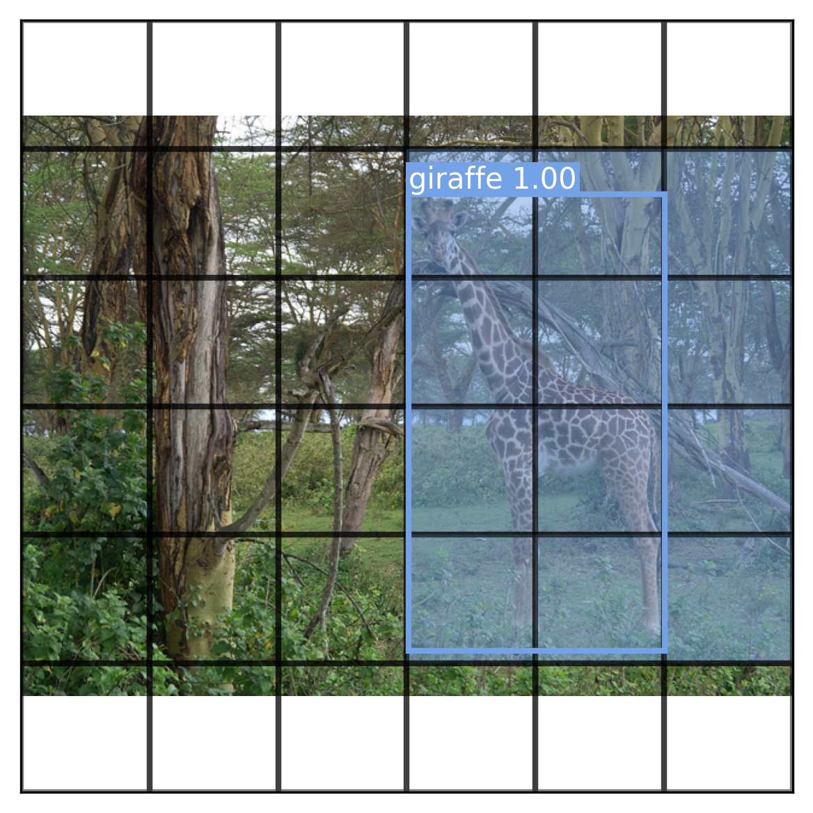
Let’s visualize our YOLO training data with our box-drawing helpers (figure 12.5). We will draw the entire class activation map over our first input image and add the confidence score of a box along with its label:

draw_prediction <- function(image, boxes, classes, cutoff = NULL) {
  draw_image(image)

1  for (yi in seq_len(grid_size)) {
    for (xi in seq_len(grid_size)) {
      label <- classes[yi, xi]
      col  <- if (label == 0) NA else label_to_color(label, alpha = 0.4)
      .[x0, y0] <- (c(xi, yi) - 1) / grid_size
      rect(
        xleft = x0, xright = x0 + 1 / grid_size,
        ytop = 1 - (y0 + 1 / grid_size), ybottom = 1 - y0,
        col = col, border = "black", lwd = 2
      )
    }
  }

2  for (yi in seq_len(grid_size)) {
    for (xi in seq_len(grid_size)) {
      cell       <- boxes[yi, xi, ]
      confidence <- cell[5]
      if (is.null(cutoff) || confidence >= cutoff) {
        grid_box <- cell[1:4]
        box <- from_grid(c(xi - 1, yi - 1), grid_box)
        label <- classes[yi, xi]
        color <- label_to_color(label)
        name <- keras_hub$utils$coco_id_to_name(label)
        draw_boxes(box, sprintf("%s %.2f", name, max(confidence, 0)), color)
      }
    }
  }
}

1: Draws the YOLO output grid and class probability map
2: Draws all boxes at each grid location above our cutoff

i <- 1
draw_prediction(
  metadata$path[i],
  box_array[i, , , ],
  class_array[i, , ],
  cutoff = 1
)

Finally, let’s use tf.data to load our image data. We will load our images from disk, apply our preprocessing, and batch them. We should also split a validation set to monitor training.

Listing 12.8: Creating a dataset to train on

library(tfdatasets, exclude = c("shape"))

images <- metadata$path |> normalizePath() |>
  tensor_slices_dataset() |>
  dataset_map(\(path) {
    path |>
1      tf$io$read_file() |>
      tf$image$decode_jpeg(channels = 3L) |>
      preprocessor()
  }, num_parallel_calls = 8)

labels <-  tensor_slices_dataset(list(
  box = box_array, class = class_array
))

2dataset <- zip_datasets(images, labels) |>
  dataset_batch(16) |> dataset_prefetch(2)

3val_dataset <- dataset |> dataset_take(500)
train_dataset <- dataset |> dataset_skip(500)

1: Loads and resizes the image with tf.data
2: Creates a merged dataset and batches it
3: Splits off some validation data

With that, our data is ready for training.

Selectively mapping the dataset into memory

This training example shows clearly why a streaming library like tf.data is helpful. Loading all the images in this large dataset in one go would overwhelm our system memory (remember, an image tensor is much larger than a compressed JPEG file). With tf.data, we can load our image data in batches and release the memory when we are done, mapping only the particular parts of the dataset we need at a given moment. The dataset_prefetch(2) call causes tf.data to keep two batches buffered and ready before they are used, so we don’t interrupt training each batch to load and resize more images.

12.2.4 Training the YOLO model

We have our model and training data ready, but we need one last element before we can actually run fit(): the loss function. Our model outputs predicted boxes and predicted grid labels. You saw in chapter 7 how to define multiple losses for each output: Keras will simply sum the losses during training. We can handle the classification loss with sparse_categorical_crossentropy as usual.

The box loss, however, needs some special consideration. The basic loss proposed by the YOLO authors is fairly simple. They used the sum-squared error of the difference between the target box parameters and the predicted ones. We will compute this error only for grid cells with actual boxes in the labeled data.

The tricky part of the loss is the box confidence output. The authors wanted the confidence output to reflect not just the presence of an object but also how good the predicted box is. To create a smooth estimate of how good a box prediction is, the authors proposed using the Intersection over Union (IoU) metric we mentioned in chapter 11. If a grid cell is empty, the predicted confidence at the location should be 0. However, if a grid cell contains an object, we can use the IoU score between the current box prediction and the actual box as the target confidence value. This way, as the model becomes better at predicting box locations, the IoU score and the learned confidence values will go up.

This calls for a custom loss function. We can start by defining a utility to compute IoU scores for target and predicted boxes.

Listing 12.9: Computing IoU for two boxes

1intersection <- function(box1, box2) {
2  .[cx1, cy1, w1, h1, conf] <- op_unstack(box1, 5, axis = -1)
  .[cx2, cy2, w2, h2, conf] <- op_unstack(box2, 5, axis = -1)

  left   <- op_maximum(cx1 - w1 / 2, cx2 - w2 / 2)
  bottom <- op_maximum(cy1 - h1 / 2, cy2 - h2 / 2)
  right  <- op_minimum(cx1 + w1 / 2, cx2 + w2 / 2)
  top    <- op_minimum(cy1 + h1 / 2, cy2 + h2 / 2)

  op_maximum(0.0, right - left) * op_maximum(0.0, top - bottom)
}

3intersection_over_union <- function(box1, box2) {
  .[cx1, cy1, w1, h1, conf] <- op_unstack(box1, 5, axis = -1)
  .[cx2, cy2, w2, h2, conf] <- op_unstack(box2, 5, axis = -1)

  inter <- intersection(box1, box2)
  a1    <- op_maximum(w1, 0.0) * op_maximum(h1, 0.0)
  a2    <- op_maximum(w2, 0.0) * op_maximum(h2, 0.0)
  union <- a1 + a2 - inter

  op_divide_no_nan(inter, union)
}

1: Computes the intersection area between two box tensors
2: Unpacks a tensor of boxes
3: Computes the IoU between two box tensors

Let’s use this utility to define our custom loss. Redmon et al. proposed a few loss-scaling tricks to improve the quality of training:

Scale up the box placement loss by a factor of five so it becomes a more important part of overall training.
Because most grid cells are empty, scale down the confidence loss in empty locations by a factor of two. This keeps these zero-confidence predictions from overwhelming the loss.
Take the square root of the width and height before computing the loss. This stops large boxes from mattering disproportionately more than small boxes. We will use a sqrt function that preserves the sign of the input, because our model may predict negative widths and heights at the start of training.

Let’s write this out.

Listing 12.10: Defining the YOLO bounding box loss

signed_sqrt <- function(x) {
  op_sign(x) * op_sqrt(op_abs(x) + config_epsilon())
}

box_loss <- function(true, pred) {
1  unpack <- \(x) list(x[.., 1:2], x[.., 3:4], x[.., 5:NA])
  .[xy_true, wh_true, conf_true] <- unpack(true)
  .[xy_pred, wh_pred, conf_pred] <- unpack(pred)

2  no_object <- conf_true == 0

3  xy_error <- op_square(xy_true - xy_pred)
  wh_error <- op_square(signed_sqrt(wh_true) - signed_sqrt(wh_pred))

4  iou <- intersection_over_union(true, pred)
  conf_target <- op_where(no_object, 0, op_expand_dims(iou, -1))
  conf_error <- op_square(conf_target - conf_pred)

5  error <- op_concatenate(axis = -1, list(
    op_where(no_object, 0, xy_error  * 5),
    op_where(no_object, 0, wh_error  * 5),
    op_where(no_object, conf_error * 0.5, conf_error)
  ))

6  op_sum(error, axis = c(2, 3, 4))
}

1: Unpacks values
2: If conf_true is 0, there is no object in this grid cell.
3: Computes box placement errors
4: Computes confidence error
5: Concatenates the errors with scaling hacks
6: Returns one loss value per sample; Keras will sum over the batch.

We are finally ready to start training our YOLO model. Purely to keep this example short, we will skip over metrics. In a real-world setting, you’d want quite a few metrics here, such as the accuracy of the model at different confidence cutoff levels.

Listing 12.11: Training the YOLO model

model |> compile(
  optimizer = optimizer_adam(2e-4),
  loss = list(box = box_loss, class = "sparse_categorical_crossentropy")
)
model |> fit(
  train_dataset,
  validation_data = val_dataset,
  epochs = 4
)

Training takes over an hour on the Colab free GPU runtime, and our model is still undertrained (validation loss is still falling!). Let’s try visualizing an output from our model (figure 12.6). We will use a low-confidence cutoff, as our model is not a very good object detector yet:

1.[x, y] <- val_dataset |> dataset_rebatch(1) |>
  as_iterator() |> iter_next()
preds <- model(x)
boxes <- preds$box@r[1, ..] |> as.array()
classes <- preds$class@r[1, ..] |>
2  op_argmax(axis = -1, zero_indexed = TRUE) |>
  as.array()
3path <- metadata[1,]$path
draw_prediction(path, boxes, classes, cutoff = 0.1)

1: Rebatches our dataset to get a single sample instead of 16
2: Uses op_argmax() to find the most likely label at each grid location
3: Loads the image from disk to view it at full size

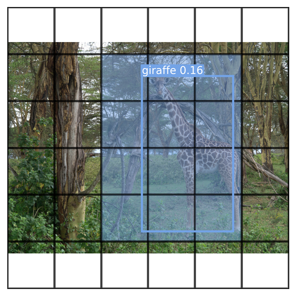
You can see that the model is starting to understand box locations and class labels, although it is still not very accurate. Let’s visualize every box predicted by the model, even those with zero confidence (figure 12.7):

draw_prediction(path, boxes, classes, cutoff = NULL)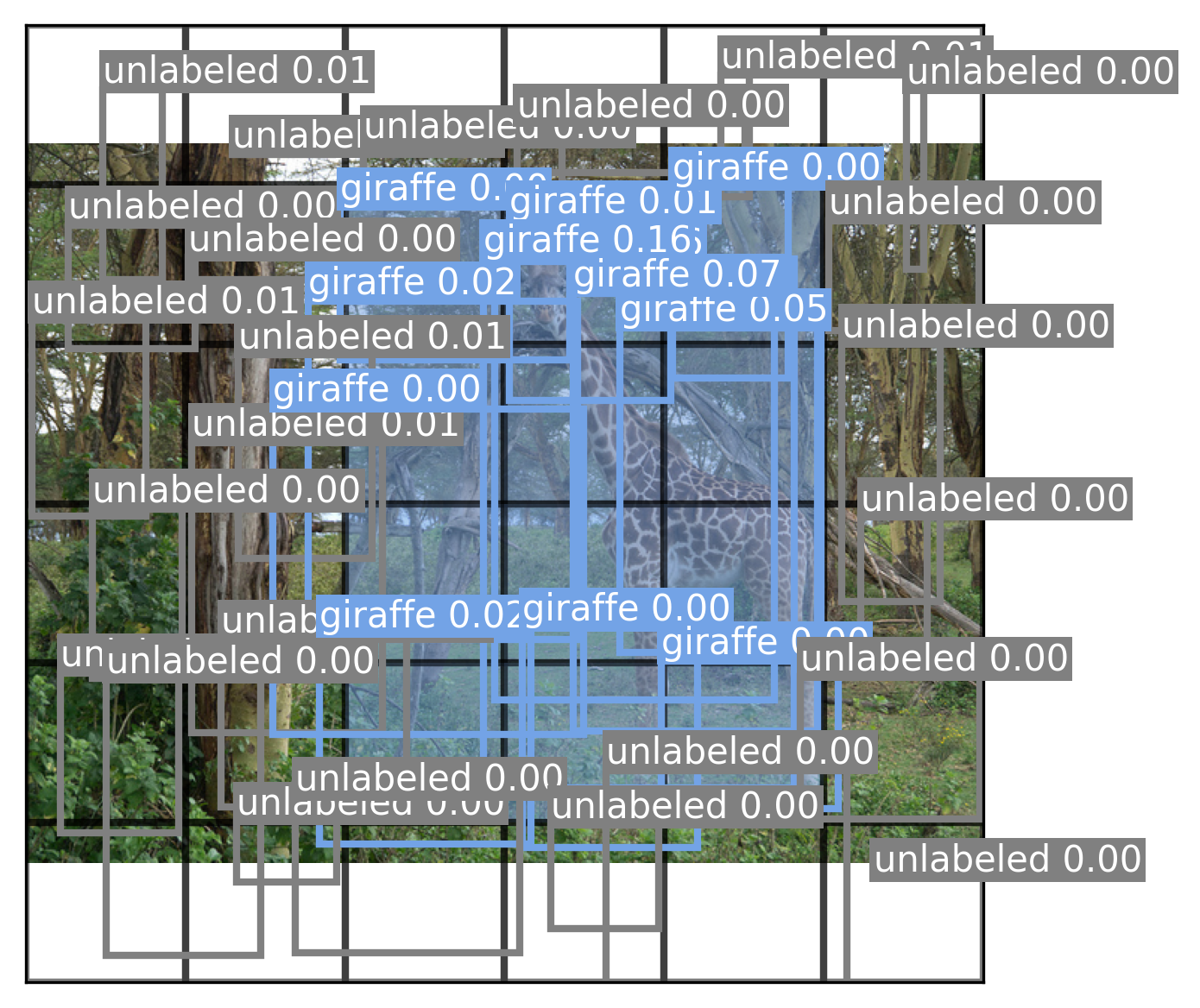

Every bounding box predicted by the YOLO model.

Our model learns very low-confidence values because it has not yet learned to consistently locate objects in a scene. To further improve the model, we can try a number of things:

Train for more epochs.
Use the entire COCO dataset.
Data augmentation (e.g., translating and rotating input images and boxes).
Improve our class probability map for overlapping boxes.
Predict multiple boxes per grid location using a bigger output grid.

All of these will positively affect model performance and get us closer to the original YOLO training recipe. However, this example is really just to get a feel for object detection training—training an accurate COCO detection model from scratch would take a large amount of compute and time. Instead, to get a sense of a better-performing detection model, let’s try using a pretrained object detection model called RetinaNet.

12.3 Using a pretrained RetinaNet detector

View on GitHub Run on Colab

RetinaNet is also a single-stage object detector and operates on the same basic principles as the YOLO model. The biggest conceptual difference between our model and RetinaNet is that RetinaNet uses its underlying convnet differently to better handle both small and large objects simultaneously.

In our YOLO model, we simply took the final outputs of our convnet and used them to build our object detector. These output features map to large areas on our input image—and as a result, they are not very effective at finding small objects in the scene.

One option to solve this scale problem would be to directly use the output of earlier layers in our convnet. This would extract high-resolution features that map to small localized areas of our input image. However, the output of these early layers is not very semantically interesting. They might map to different types of simple features like edges and curves, but only later in the convnet layers do we start building latent representations for entire objects.

The solution used by RetinaNet is called a feature pyramid network (FPN). The final features from the convnet base model are upsampled with progressive Conv2DTranspose layers, just as you saw in the previous chapter. But, critically, we also include lateral connections where we sum these upsampled feature maps with the feature maps of the same size from the original convnet. This combines the semantically interesting, low-resolution features at the end of the convnet with the high-resolution, small-scale features from the beginning of the convnet. A rough sketch of this architecture is shown in figure 12.8.

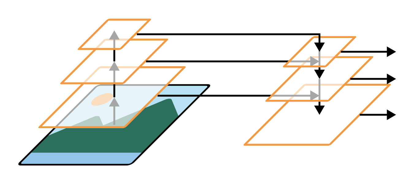
An FPN creates semantically interesting feature maps at different scales.

FPNs can substantially boost performance by building effective features for both small and large objects in terms of pixel footprint. Recent versions of YOLO also use the same setup.

Let’s try out the RetinaNet model, which was also trained on the COCO dataset. To make this a little more interesting, let’s use an image that is out of distribution for the model: the Pointillist painting A Sunday Afternoon on the Island of La Grande Jatte.

We can start by downloading the image and converting it to a NumPy array:

url <- paste0(
  "https://upload.wikimedia.org/wikipedia/commons/thumb/7/7d/",
  "A_Sunday_on_La_Grande_Jatte%2C_Georges_Seurat%2C_1884.jpg/",
  "1280px-A_Sunday_on_La_Grande_Jatte%2C_Georges_Seurat%2C_1884.jpg"
)
path <- get_file("la_grande_jatte.jpg", origin = url)
image <- image_load(path) |> image_to_array(dtype = "float32")

Next, let’s download the model and make a prediction. As we did in chapter 11, we can use the high-level task API in KerasHub to create an ObjectDetector and use it—preprocessing included.

Listing 12.12: Creating the ObjectDetector model

detector <- keras_hub$models$ObjectDetector$from_preset(
  "retinanet_resnet50_fpn_v2_coco",
  bounding_box_format =  "rel_xywh"
)
1predictions <- predict(detector, list(image))

1: list(image) is a trick for adding a batch dimension.

You’ll note that we pass an extra argument to specify the bounding box format. We can do this for most Keras models and layers that support bounding boxes. We pass "rel_xywh" to use the same format as we did for the YOLO model, so we can use the same box drawing utilities. Here, rel stands for relative to the image size (e.g., from [0, 1]). Let’s inspect the prediction we just made:

str(predictions)

List of 4
 $ boxes         : num [1, 1:100, 1:4] 0.0275 0.2892 0.7349 0.627 0.4325 ...
 $ confidence    : num [1, 1:100] 0.692 0.659 0.65 0.632 0.603 ...
 $ labels        : int [1, 1:100] 1 1 1 1 1 18 1 28 28 1 ...
 $ num_detections: int [1(1d)] 11

We have four different model outputs: bounding boxes, confidences, labels, and the total number of detections. This is overall similar to our YOLO model. The model can predict a total of 100 objects for each input image.

Let’s display the prediction with our box-drawing utilities (figure 12.9).

Listing 12.13: Running inference with RetinaNet

draw_image(path, show_padding = FALSE)
for(i in seq_len(predictions$num_detections)) {
  box <- predictions$boxes[1, i, ] |> matrix(ncol = 4)
  colnames(box) <- c("left", "top", "width", "height")
  label <- predictions$labels[1, i]
  label_name <- keras_hub$utils$coco_id_to_name(label)
  draw_boxes(box, label_name, label_to_color(label))
}

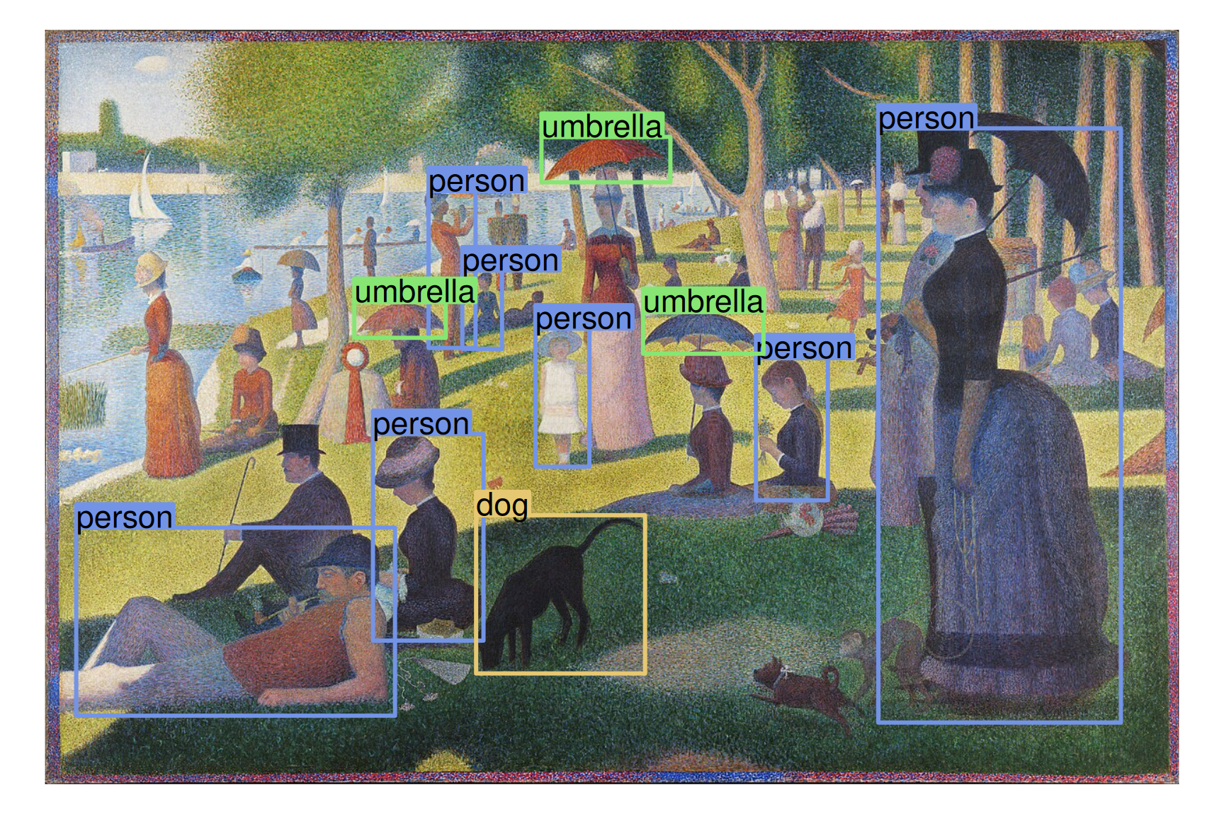
RetinaNet detections for A Sunday Afternoon on the Island of La Grande Jatte. — RetinaNet detections for *A Sunday Afternoon on the Island of La Grande Jatte*.⁴

The RetinaNet model is able to generalize to a Pointillist painting with ease, despite no training on this style of input! This is one of the advantages of single-stage object detectors. Paintings and photographs are very different at a pixel level but share a similar structure at a high level. Two-stage detectors like R-CNNs are forced to classify small patches of an input image in isolation, which is extra difficult when small patches of pixels look very different from the training data. But single-stage detectors can draw on features from the entire input and are more robust to novel test-time inputs.

With that, you have reached the end of the computer vision section of this book! You have trained image classifiers, segmenters, and object detectors from scratch. And you’ve developed a good intuition for how convnets work, the first major success of the deep learning era. We aren’t quite done with images yet; you will see them again in chapter 17 when we start generating image output.

12.4 Summary

Object detection identifies and locates objects within an image using bounding boxes. It’s basically a weaker version of image segmentation, but one that can be run much more efficiently.
There are two primary approaches to object detection:
- Region-based convolutional neural networks (R-CNNs), which are two-stage models that first propose regions of interest and then classify them with a convnet.
- Single-stage detectors (like RetinaNet and YOLO), which perform both tasks in a single step. Single-stage detectors are generally faster and more efficient, making them suitable for real-time applications (e.g., self-driving cars).
YOLO computes two separate outputs simultaneously during training—possible bounding boxes and a class probability map:
- Each candidate bounding box is paired with a confidence score, which is trained to target the Intersection over Union of the predicted box and the ground truth box.
- The class probability map classifies different regions of an image as belonging to different objects.
RetinaNet builds on this idea by using a feature pyramid network (FPN), which combines features from multiple convnet layers to create feature maps at different scales, allowing it to more accurately detect objects of different sizes.

Image from the COCO 2017 dataset, https://cocodataset.org/. Image from Flickr, http://farm8.staticflickr.com/7250/7520201840_3e01349e3f_z.jpg, CC BY 2.0 https://creativecommons.org/licenses/by/2.0/.↩︎
“You Only Look Once: Unified, Real-Time Object Detection” [2015], https://arxiv.org/abs/1506.02640 ↩︎
Image from the COCO 2017 dataset, https://cocodataset.org/. Image from Flickr, http://farm9.staticflickr.com/8081/8387882360_5b97a233c4_z.jpg, CC BY 2.0 https://creativecommons.org/licenses/by/2.0/.↩︎
Image: Georges Seurat, public domain, via Wikimedia Commons, https://commons.wikimedia.org/wiki/File:A_Sunday_on_La_Grande_Jatte,_Georges_Seurat,_1884.jpg.↩︎