14 Text classification

This chapter covers

An introduction to the field of natural language processing (NLP)
Preprocessing text input into numeric input
Building simple text classification models

This chapter will lay the foundation for working with text input that we will build on in the next two chapters of this book. By the end of this chapter, you will be able to build a simple text classifier in a number of different ways. This will set the stage for building more complicated models, like the Transformer, in the next chapter.

14.1 A brief history of natural language processing

In computer science, we refer to human languages, like English or Mandarin, as “natural” languages to distinguish them from languages that were designed for machines, like LISP, Assembly, and XML. Every machine language was designed: its starting point was an engineer writing down a set of formal rules to describe what statements we can make and what they mean. The rules came first, and people only started using the language once the ruleset was complete. With human language, it’s the reverse: usage comes first, and rules arise later. Natural language was shaped by an evolutionary process, much like biological organisms—that’s what makes it “natural.” Its “rules,” like the grammar of English, were formalized after the fact and are often ignored or broken by its users. As a result, whereas machine-readable language is highly structured and rigorous, natural language is messy—ambiguous, chaotic, sprawling, and constantly in flux.

Computer scientists have long fixated on the potential of systems that can ingest or produce natural language. Language, particularly written text, underpins most of our communications and cultural production. Centuries of human knowledge are stored via text; the internet is mostly text, and even our thoughts are based on language! The practice of using computers to interpret and manipulate language is called natural language processing (NLP). It was first proposed as a field of study immediately following World War II, when some thought we could view understanding language as a form of “code cracking,” where natural language is the “code” used to transmit information.

In the early days of the field, many people naively thought that we could write down the “rule set of English,” much like one can write down the rule set of LISP. In the early 1950s, researchers at IBM and Georgetown demonstrated a system that could translate Russian into English. The system used a grammar with six hardcoded rules and a lookup table with a couple of hundred elements (words and suffixes) to translate 60 handpicked Russian sentences accurately. The goal was to drum up excitement and funding for machine translation, and in that sense, it was a huge success. Despite the limited nature of the demo, the authors claimed that within five years, translation would be a solved problem. Funding poured in for the better part of a decade. However, generalizing such a system proved to be maddeningly difficult. Words change their meaning dramatically depending on context. Any grammar rules needed countless exceptions. Developing a program that could shine on a few handpicked examples was simple enough, but building a robust system that could compete with human translators was another matter. An influential US report, a decade later, picked apart the lack of progress, and funding dried up.

Despite these setbacks and repeated swings from excitement to disillusionment, handcrafted rules held out as the dominant approach well into the 1990s. The problems were obvious, but there was simply no viable alternative to writing down symbolic rules to describe grammar. However, as faster computers and greater quantities of data became available in the late 1980s, research began to head in a new direction. When you find yourself building systems that are big piles of ad hoc rules, as a clever engineer, you’re likely to start asking, “Could I use a corpus of data to automate the process of finding these rules? Could I search for the rules within some rule space, instead of having to come up with them myself?” And just like that, you’ve graduated to doing machine learning.

In the late 1980s, we started seeing machine learning approaches to natural language processing. The earliest ones were based on decision trees: the intent was literally to automate the development of the kind of if/then/else rules of hardcoded language systems. Then statistical approaches started gaining speed, beginning with logistic regression. Over time, learned parametric models took over, and linguistics came to be seen by some as a hindrance when baked directly into a model. Frederick Jelinek, an early speech recognition researcher, joked in the 1990s, “Every time I fire a linguist, the performance of the speech recognizer goes up.”

Much as computer vision is pattern recognition applied to pixels, the modern field of NLP is all about pattern recognition applied to words in text. There’s no shortage of practical applications:

Given the text of an email, what is the probability that it is spam? (text classification)
Given an English sentence, what is the most likely Russian translation? (translation)
Given an incomplete sentence, what word will likely come next? (language modeling)

The text-processing models we will train in this book won’t possess a human-like understanding of language; rather, they simply look for statistical regularities in their input data, which turns out to be sufficient to perform well on a wide array of real-world tasks.

In the last decade, NLP researchers and practitioners have discovered just how shockingly effective it can be to learn the answer to narrow statistical questions about text. In the 2010s, researchers began applying LSTM models to text, dramatically increasing the number of parameters in NLP models and the compute resources required to train them. The results were encouraging: LSTMs could generalize to unseen examples with far greater accuracy than previous approaches, but they eventually hit limits. LSTMs struggled to track dependencies in long chains of text with many sentences and paragraphs, and compared to computer vision models, they were slow and unwieldy to train.

Toward the end of the 2010s, researchers at Google discovered a new architecture called the Transformer that solved many scalability problems plaguing LSTMs. As long as they increased the size of a model and its training data together, Transformers appeared to perform more and more accurately. Better yet, the computations needed for training a Transformer could be effectively parallelized, even for long sequences. If we doubled the number of machines doing training, we could roughly halve the time we need to wait for a result.

The discovery of the Transformer architecture, along with ever-faster GPUs and CPUs, has led to a dramatic explosion of investment and interest in NLP models over the past few years. Chat systems like ChatGPT have captivated public attention with their ability to produce fluent and natural text on seemingly arbitrary topics and questions. The raw text used to train these models is a significant portion of all written language available on the internet, and the compute to train individual models can cost tens of millions of dollars. Some hype is worth cutting down to size: these are pattern recognition machines. Despite our persistent human tendency to find intelligence in “things that talk,” these models copy and synthesize training data in a way that is wholly distinct from (and much less efficient than!) human intelligence. However, it is also fair to say that the emergence of complex behaviors from incredibly simple “guess the missing word” training setups has been one of the most shocking empirical results in the last decade of machine learning.

In the following three chapters, we will look at a range of techniques for machine learning with text data. We will skip discussion of the hardcoded linguistic features that prevailed until the 1990s, but we will look at everything from running logistic regressions for classifying text to training LSTMs for machine translation. We will closely examine the Transformer model and discuss what makes it so scalable and effective at generalizing in the text domain. Let’s dig in.

14.2 Preparing text data

Let’s consider an English sentence:

text <- "The quick brown fox jumped over the lazy dog."

There is an obvious blocker before we can start applying any of the deep learning techniques of previous chapters: our input is not numeric! Before beginning any modeling, we need to translate the written word into tensors of numbers. Unlike images, which have a relatively natural numeric representation, we can build a numeric representation of text in several ways.

A simple approach would be to borrow from standard text file formats for text and use something like an ASCII encoding. We could chop the input into a sequence of characters and assign each a unique index. Another intuitive approach would be to build a representation based on words, first breaking sentences apart at all spaces and punctuation and then mapping each word to a unique numeric representation.

These are both good approaches to try, and in general, all text preprocessing will include a splitting step, where text is split into small, individual units called tokens. A powerful tool for splitting text is regular expressions, which can flexibly match patterns of characters in text.

Learning regex

Regular expressions are an incredibly powerful and versatile way to express string operations.

If you are unfamiliar with them, they are well worth the effort to learn, but teaching regex is outside the scope of this book. A great place to start is https://stringr.tidyverse.org/articles/regular-expressions.html.

If you’re working with base R string processing functions like grep(), be sure to also check out the base R man page at help(regex, base).

Let’s look at how to use the stringr package to split a string into a sequence of characters. The most basic approach is to use the built-in boundary() function, which can identify all character start and stop positions in the string:

library(stringr)
library(glue)
library(dplyr)
library(keras3)

split_chars <- function(text) {
  unlist(str_split(text, boundary("character")))
}

We can apply the function to our example input string.

"The quick brown fox jumped over the lazy dog." |>
  split_chars() |> head(12)

 [1] "T" "h" "e" " " "q" "u" "i" "c" "k" " " "b" "r"

The boundary() function can also identify word boundaries. We can use this to split our text into words instead. By default, boundary("word") will discard punctuation characters like .!?;. To preserve these, we need to take two steps. First, we call boundary() with skip_word_none = FALSE to keep non-word elements in the output. This will preserve punctuation and also whitespace between words. Next, we subset the returned character vector to keep only strings that match the regex \\S: the negation of \\s, which matches whitespace. In other words, we keep all elements that are not just whitespace:

split_words <- function(text) {
  text |>
    str_split(boundary("word", skip_word_none = FALSE)) |>
    unlist() |>
    str_subset("\\S")
}

Splitting text in stringr

There are a few ways to split text in stringr, and they serve different purposes:

Use str_split(x, "") (or str_split(x, boundary("character"))) to split into individual characters. In stringr, these two are equivalent and Unicode-aware.
Use str_split(x, boundary("word")) to split into words using ICU’s word-boundary rules. By default, this drops punctuation and whitespace. If you want to keep punctuation too, use boundary("word", skip_word_none = FALSE) and then filter out whitespace tokens as we do in split_words().
The regex pattern "\\b" (a regex word boundary) splits at transitions between word characters (letters/digits/underscore) and non-word characters. It can split contractions like "don't" into pieces and may yield empty tokens at the start or end of a string, so it isn’t a drop-in replacement for boundary("word").

Here’s what it does to a test sentence:

split_words("The quick brown fox jumped over the dog.")

[1] "The"    "quick"  "brown"  "fox"    "jumped" "over"   "the"    "dog"   
[9] "."

Splitting takes us from a single string to a token sequence, but we still need to transform our string tokens into numeric inputs. By far the most common approach is to map each token to a unique integer index, often called indexing our input. This is a flexible and reversible representation of our tokenized input that can work with a wide range of modeling approaches. Later on, we can decide how to map from token indices into a latent space ingested by the model.

For character tokens, we could use ASCII lookups to index each token: for example, utf8ToInt('A') → 65 and utf8ToInt('z') → 122. However, this approach can scale poorly when we start to consider other languages—there are more than a million characters in the Unicode specification! A more robust technique is to build a mapping from specific tokens in our training data to indices that occur in the data we care about, which in NLP is called a vocabulary. This has the nice property of working for word-level tokens as easily as character-level tokens.

Let’s take a look at how we might use a vocabulary to transform text. We will build a simple character vector of tokens and use the index positions of tokens in the vector as the indices:

vocabulary <- c("the", "quick", "brown", "fox", "jumped", "over", "dog", ".")
words <- split_words("The quick brown fox jumped over the lazy dog.")
indices <- match(words, vocabulary, nomatch = 0L)
indices

 [1] 0 2 3 4 5 6 1 0 7 8

Note that for words not in the vocabulary, we use 0 as their index. Later, we’ll map 0 back to a special token called "[UNK]", which represents a token unknown to the vocabulary. This allows us to index all input we encounter, even if some terms appear only in the test data. In the previous example, "lazy" maps to the "[UNK]" index 0 because it wasn’t included in our vocabulary.

With these simple text transformations, we are well on our way to building a text preprocessing pipeline. However, there is one more common type of text manipulation we should consider: standardization. Consider these two sentences:

“sunset came. i was staring at the Mexico sky. Isnt nature splendid??”
“Sunset came; I stared at the México sky. Isn’t nature splendid?”

They are very similar—in fact, they are almost identical. Yet if we were to convert them to indices as previously described, we would end up with very different representations because “i” and “I” are two distinct characters, “Mexico” and “México” are two distinct words, “isnt” isn’t “isn’t,” and so on. A machine learning model doesn’t know a priori that “i” and “I” are the same letter, that “é” is an “e” with an accent, or that “staring” and “stared” are two forms of the same verb. Standardizing text is a basic form of feature engineering that aims to erase encoding differences that we don’t want our model to have to deal with. It’s not exclusive to machine learning, either—we’d have to do the same thing if we were building a search engine.

One simple and widespread standardization scheme is to convert to lowercase and remove punctuation characters. Our two sentences would become

“sunset came i was staring at the mexico sky isnt nature splendid”
“sunset came i stared at the méxico sky isnt nature splendid”

Much closer already. We could get even closer if we removed accent marks from all characters.

There’s a lot we can do with standardization, and it used to be one of the most critical areas to improve model performance. For many decades in NLP, it was common practice to use regular expressions to attempt to map words to a common root (e.g., “tired” → “tire” and “trophies” → “trophy”), called stemming or lemmatization. But as models have grown more expressive, this type of standardization tends to do more harm than good. The tense and plurality of a word are necessary signals to its meaning. For the larger models used today, most standardization is as light as possible—for example, converting all inputs to a standard character encoding before further processing.

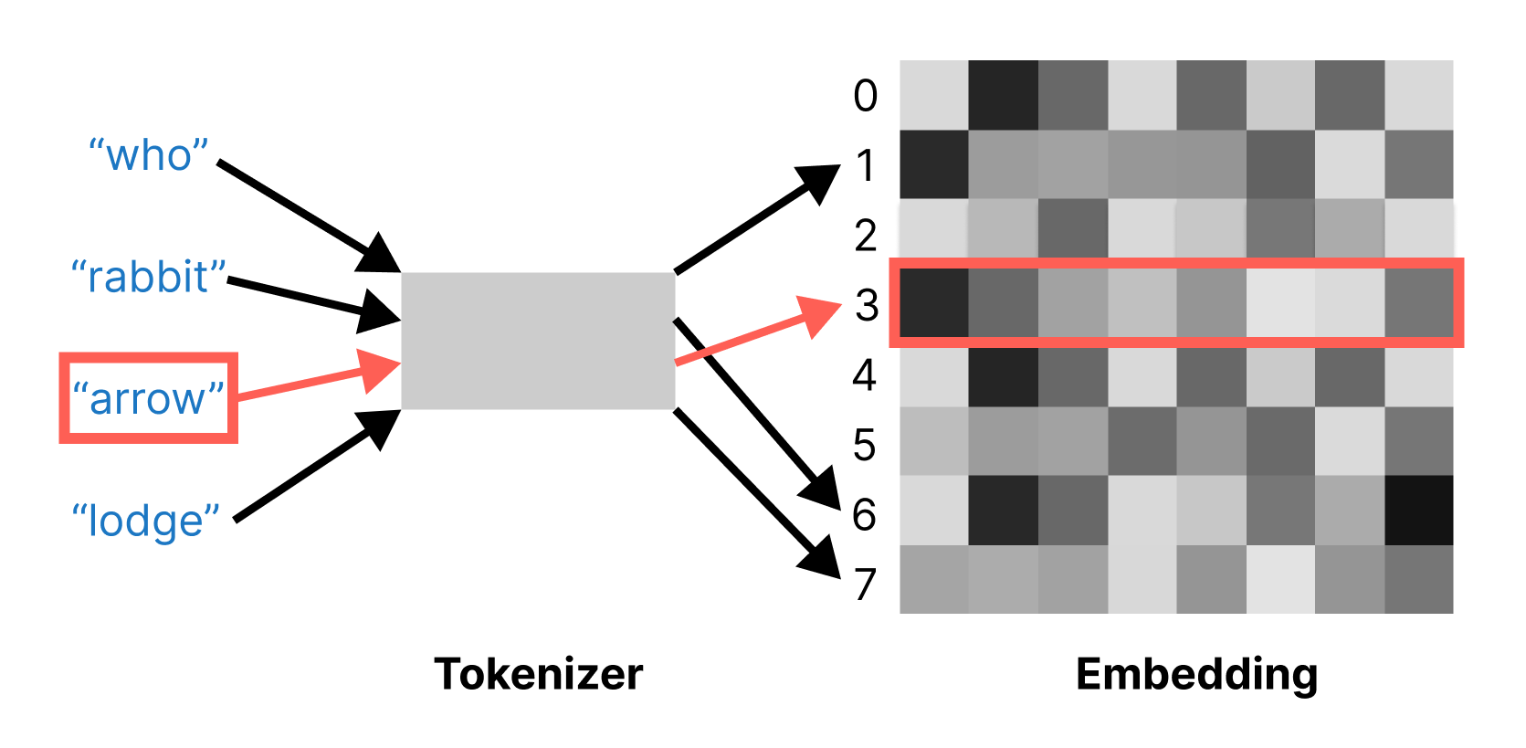
With standardization, we have now seen three distinct stages for preprocessing text (figure 14.1):

Standardization—Normalizes input with basic text-to-text transformations
Splitting—Splits text into sequences of tokens
Indexing—Maps tokens to indices using a vocabulary

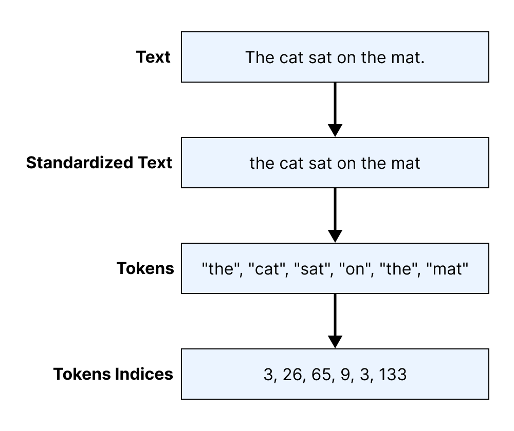
People often refer to the entire process as tokenization and to an object that maps text to a sequence of token indices as a tokenizer. Let’s try building a few.

14.2.1 Character and word tokenization

To start, let’s build a character-level tokenizer that maps each character in an input string to an integer. To keep things simple, we will use only one standardization step: lowercasing all input.

Listing 14.1: A basic character-level tokenizer.

new_char_tokenizer <- function(vocabulary, nomatch = "[UNK]") {
  self <- new.env(parent = emptyenv())
  attr(self, "class") <- "CharTokenizer"

  self$vocabulary <- vocabulary
  self$nomatch <- nomatch

  self$standardize <- function(strings) {
    str_to_lower(strings)
  }

  self$split <- function(strings) {
    split_chars(strings)
  }

  self$index <- function(tokens) {
    match(tokens, self$vocabulary, nomatch = 0L)
  }

1  self$tokenize <- function(strings) {
    strings |>
      self$standardize() |>
      self$split() |>
      self$index()
  }

2  self$detokenize <- function(indices) {
    indices[indices == 0] <- NA
    matches <- self$vocabulary[indices]
    matches[is.na(matches)] <- self$nomatch
    matches
  }

  self
}

1: Encodes string to integers
2: Decodes integers to strings

Pretty simple. Before using this, we also need to build a function that computes a vocabulary of tokens based on some input text. Rather than simply mapping all characters to a unique index, let’s give ourselves the ability to limit our vocabulary size to only the most common tokens in our input data. When we get into the modeling side of things, limiting the vocabulary size will be an important way to limit the number of parameters in a model.

Listing 14.2: Computing a character-level vocabulary.

compute_char_vocabulary <- function(inputs, max_size = Inf) {
  tibble(chars = split_chars(inputs)) |>
    count(chars, sort = TRUE) |>
    slice_head(n = max_size) |>
    pull(chars)
}

We can now do the same for a word-level tokenizer. We can use the same code as our character-level tokenizer with a different splitting step.

Listing 14.3: A basic word-level tokenizer.

new_word_tokenizer <- function(vocabulary, nomatch = "[UNK]") {
  self <- new.env(parent = emptyenv())
  attr(self, "class") <- "WordTokenizer"

1  vocabulary; nomatch;

  self$standardize <- function(string) {
    tolower(string)
  }

  self$split <- function(inputs) {
    split_words(inputs)
  }

  self$index <- function(tokens) {
    match(tokens, vocabulary, nomatch = 0)
  }

2  self$tokenize <- function(string) {
    string |>
      self$standardize() |>
      self$split() |>
      self$index()
  }

3  self$detokenize <- function(indices) {
    indices[indices == 0] <- NA
    matches <- vocabulary[indices]
    matches[is.na(matches)] <- nomatch
    matches
  }

  self
}

1: Forces R promises. These will be private variables.
2: Encodes strings to integers
3: Decodes integers to strings

We can also substitute this new split rule into our vocabulary function.

Listing 14.4: Computing a word-level vocabulary.

compute_word_vocabulary <- function(inputs, max_size) {
  tibble(words = split_words(inputs)) |>
    count(words, sort = TRUE) |>
    slice_head(n = max_size) |>
    pull(words)
}

Let’s try out our tokenizers on some real-world input: the full text of Moby Dick by Herman Melville. We will first build a vocabulary for both tokenizers and then use it to tokenize some text:

filename <- get_file(
  origin = "https://www.gutenberg.org/files/2701/old/moby10b.txt"
)
moby_dick <- readLines(filename)

vocabulary <- compute_char_vocabulary(moby_dick, max_size = 100)
char_tokenizer <- new_char_tokenizer(vocabulary)

Let’s inspect what our character-level tokenizer has computed:

str(vocabulary)

 chr [1:89] " " "e" "t" "a" "o" "n" "s" "i" "h" "r" "l" "d" "u" "m" "c" ...

head(vocabulary, 10)

 [1] " " "e" "t" "a" "o" "n" "s" "i" "h" "r"

tail(vocabulary, 10)

 [1] "@" "$" "%" "#" "&" "=" "~" "+" "<" ">"

Now, what about the word-level tokenizer?

vocabulary <- compute_word_vocabulary(moby_dick, max_size = 2000)
word_tokenizer <- new_word_tokenizer(vocabulary)

We can print out the same data for our word-level tokenizer:

str(vocabulary)

 chr [1:2000] "," "the" "." "of" "and" "-" "a" "to" ";" "in" "\"" ...

tail(vocabulary)

[1] "fowls"  "freely" "ginger" "grim"   "hearse" "hell"

string <- "Call me Ishmael. Some years ago--never mind how long precisely."
tokenized <- word_tokenizer$tokenize(string)
str(tokenized)

 int [1:15] 445 46 0 3 53 264 631 6 6 152 ...

tokenized |>
  word_tokenizer$detokenize() |>
  str_flatten(collapse = " ")

[1] "call me [UNK] . some years ago - - never mind how long precisely ."

You can already see some of the strengths and weaknesses of both tokenization techniques. A character-level tokenizer needs only 89 vocabulary terms to cover the entire book but will encode each input as a very long sequence. A word-level tokenizer quickly fills a 2,000-term vocabulary (we would need a dictionary with 17,000 terms to index every word in the book!), but the outputs of the word-level tokenizer are much shorter.

As machine learning practitioners have scaled models up with more and more data and parameters, the downsides of both word and character tokenization have become apparent. The “compression” offered by word-level tokenization turns out to be very important—it lets us feed longer sequences into a model. However, if we attempt to build a word-level vocabulary for a large dataset (today, we might see a dataset with trillions of words), we would have an unworkably large vocabulary with hundreds of millions of terms. If we aggressively restrict our word-level vocabulary size, we will encode a lot of text to the "[UNK]" token, throwing out valuable information. These problems have led to the rise in popularity of a third type of tokenization, called subword tokenization, which attempts to bridge the gap between word- and character-level approaches.

14.2.2 Subword tokenization

Subword tokenization aims to combine the best of both character- and word-level encoding techniques. We want the WordTokenizer’s ability to produce concise output and the CharTokenizer’s ability to encode a wide range of inputs with a small vocabulary.

You can think of the search for the ideal tokenizer as the hunt for an ideal compression of the input data. Reducing the token length compresses the overall length of our examples. A small vocabulary reduces the number of bytes required to represent each token. If we achieve both, we will be able to feed short, information-rich sequences to our deep learning model.

This analogy between compression and tokenization was not always obvious, but it turns out to be powerful. One of the most practically effective tricks found in the last decade of NLP research was repurposing a 1990s algorithm for lossless compression called byte-pair encoding¹ for tokenization. It is used by ChatGPT and many other models to this day. In this section, we will build a tokenizer that uses the byte-pair encoding algorithm.

The idea with byte-pair encoding is to start with a basic vocabulary of characters and progressively “merge” common pairings into longer and longer sequences of characters. Let’s say we start with the following input text:

data <- c(
  "the quick brown fox",
  "the slow brown fox",
  "the quick brown foxhound"
)

To apply byte-pair encoding to our text, we first split the text into individual characters. Then we tokenize the text and count how often each pair of adjacent tokens appears within words:

count_pairs <- function(tokens) {
  tibble(left = tokens, right = lead(tokens)) |>
    count(left, right, sort = TRUE) |>
    filter(left != " " & right != " ")
}

data |> split_chars() |> count_pairs()

# A tibble: 20 × 3
   left  right     n
   <chr> <chr> <int>
 1 o     w         4
 2 b     r         3
 3 f     o         3
 4 h     e         3
 5 o     x         3
 6 r     o         3
 7 t     h         3
 8 w     n         3
 9 c     k         2
10 i     c         2
11 q     u         2
12 u     i         2
13 x     t         2
14 h     o         1
15 l     o         1
16 n     d         1
17 o     u         1
18 s     l         1
19 u     n         1
20 x     h         1

To apply byte-pair encoding to our split word counts, we will find two characters and merge them into a new symbol. We’ll consider all pairs of characters in all words and merge only the most common one we find. In the previous example, the most common character pair is ("o", "w"), in both the word "brown" (which occurs three times in our data) and "slow" (which occurs once). We combine this pair into a new symbol "ow" and merge all occurrences of "ow".

Then we continue, counting pairs and merging pairs, except now "ow" will be a single unit that could merge with, say, "l" to form "low". By progressively merging the most frequent symbol pair, we build up a vocabulary of larger and larger subwords.

Let’s try this out on our toy dataset:

get_most_common_pair <- function(tokens) {
  count_pairs(tokens) |>
    slice_max(n, with_ties = FALSE) |>
    select(left, right)
}

merge_pair <- function(tokens, pair) {
  matches <- which(
    tokens == pair$left & lead(tokens) == pair$right
  )

  tokens[matches] <- str_c(tokens[matches], tokens[matches + 1])
  tokens <- tokens[-(matches + 1)]
  tokens
}

show_tokens <- function(prefix, tokens) {
  tokens <- str_flatten(c("", unique(unlist(tokens)), ""), collapse = "_")
  cat(prefix, ": ", tokens, "\n", sep = "")
}

tokens <- data |> split_chars()
show_tokens(0, tokens)
for (i in seq_len(9)) {
  pair <- get_most_common_pair(tokens)
  tokens <- tokens |> merge_pair(pair)
  show_tokens(i, tokens)
}

0: _t_h_e_ _q_u_i_c_k_b_r_o_w_n_f_x_s_l_d_
1: _t_h_e_ _q_u_i_c_k_b_r_ow_n_f_o_x_s_l_d_
2: _t_h_e_ _q_u_i_c_k_br_ow_n_f_o_x_s_l_d_
3: _t_h_e_ _q_u_i_c_k_brow_n_f_o_x_s_l_ow_d_
4: _t_h_e_ _q_u_i_c_k_brown_f_o_x_s_l_ow_n_d_
5: _t_h_e_ _q_u_i_c_k_brown_fo_x_s_l_ow_o_n_d_
6: _t_h_e_ _q_u_i_c_k_brown_fox_s_l_ow_o_n_d_
7: _t_he_ _q_u_i_c_k_brown_fox_s_l_ow_h_o_n_d_
8: _the_ _q_u_i_c_k_brown_fox_s_l_ow_h_o_n_d_
9: _the_ _q_u_i_ck_brown_fox_s_l_ow_h_o_n_d_

You can see how common words are merged entirely, whereas less common words are only partially merged.

We can now extend this to a full function for computing a byte-pair encoding vocabulary. We start our vocabulary with all characters found in the input text, and we will progressively add merged symbols (larger and larger subwords) to our vocabulary until it reaches our desired length. We also keep a separate list of our merge rules in the order in which we applied them. Next, we will see how to use these merge rules to tokenize new input text.

Listing 14.5: Computing a byte-pair encoding vocabulary.

compute_sub_word_vocabulary <- function(dataset, vocab_size) {
  dataset <- split_chars(dataset)
  vocab <- compute_char_vocabulary(dataset)
  merges <- list()
  while (length(vocab) < vocab_size) {
    pair <- get_most_common_pair(dataset)
    nrow(pair) || break
    dataset <- dataset |> merge_pair(pair)
    new_token <- str_flatten(pair)
    merges[[length(merges) + 1]] <- pair
    vocab[[length(vocab) + 1]] <- new_token
  }
  list(vocab = vocab, merges = merges)
}

Let’s build a SubWordTokenizer that applies our merge rules to tokenize new input text. The standardize() and index() steps can stay the same as in the WordTokenizer, with all changes coming in the split() method.

In our splitting step, we first split all input into characters. Next, we iterate over the merge pairs and successively apply our learned merge rules to the split characters. As an implementation detail, we do this by temporarily flattening the entire dataset into a single string and then using str_replace_all(). This allows us to efficiently apply all merge rules using string substitution.

After bpe_merge(), what is returned are “subwords”: tokens that may be entire words, partial words, or simple characters, depending on the input word’s frequency in our training data. These subwords are tokens in our output.

Listing 14.6: A byte-pair encoding tokenizer.

bpe_merge <- function(data, merges) {
1  sep <- "|||SEP|||"
  data <- str_flatten(data, collapse = sep)
2  for (pair in merges) {
    .[left, right] <- pair
3    data <- data |> str_replace_all(
      pattern = fixed(str_c(sep, left, sep, right, sep)),
      replacement = str_c(sep, left, right, sep)
    )
  }
4  str_split_1(data, fixed(sep))
}

1: Temporarily flattens into a single string with a unique separator
2: Applies merge rules in “rank” order. More frequent pairs are merged first.
3: Uses string substitution to remove sep between merge pairs
4: Splits flattened string back into tokens

new_subword_tokenizer <- function(vocabulary, merges, nomatch = "[UNK]") {
  self <- new.env(parent = emptyenv())
  attr(self, "class") <- "SubWordTokenizer"

  vocabulary; merges; nomatch

  self$standardize <- function(string) {
    tolower(string)
  }

  self$split <- function(string) {
    string |> split_chars() |> bpe_merge(merges)
  }

  self$index <- function(tokens) {
    match(tokens, vocabulary, nomatch = 0)
  }

  self$tokenize <- function(string, nomatch = 0) {
    string |>
      self$standardize() |>
      self$split() |>
      self$index()
  }

  self$detokenize <- function(indices) {
    indices[indices == 0] <- NA
    matches <- vocabulary[indices]
    matches[is.na(matches)] <- nomatch
    matches
  }

  self
}

Let’s try out our tokenizer on the full text of Moby Dick:

1.[vocabulary, merges] <- compute_sub_word_vocabulary(moby_dick, 2000)
sub_word_tokenizer <- new_subword_tokenizer(vocabulary, merges)

1: This can take a few minutes.

We can take a look at our vocabulary and try a test sentence on our tokenizer, as we did with WordTokenizer and CharTokenizer:

str(vocabulary)

 chr [1:2000] " " "e" "t" "a" "o" "n" "s" "i" "h" "r" "l" "d" "u" "m" ...

tail(vocabulary)

[1] "ience"  "infer"  "ise,"   "island" "ivid"   "lau"

tokenized <- sub_word_tokenizer$tokenize(string)
str(tokenized)

 int [1:27] 15 129 1 220 1 236 1110 158 25 1 ...

tokenized |> sub_word_tokenizer$detokenize() |> str_flatten("_")

[1] "c_all_ _me_ _ish_ma_el_._ _some_ _years_ _ago_--_never_ _mind_ _how_ _long_ _precise_ly_."

The SubWordTokenizer has a slightly longer length for our test sentence than the WordTokenizer (16 vs. 13 tokens), but unlike the WordTokenizer, it can tokenize every word in Moby Dick without using the "[UNK]" token. The vocabulary contains every character in our source text, so the worst-case performance will be tokenizing a word into individual characters. We have achieved a short average token length while handling rare words with a small vocabulary. This is the advantage of subword tokenizers.

You might notice that running this code is noticeably slower than the word and character tokenizers; it takes about a minute on our reference hardware. Learning merge rules is much more complex than simply counting the words in an input dataset. Although this is a downside to subword tokenization, it is rarely an important concern in practice. We need to learn a vocabulary only once per model, and the cost of learning a subword vocabulary is generally negligible compared to model training.

One final note on tokenization: although it is important to understand how tokenizers work, you will rarely need to build one yourself. Keras comes with utilities for tokenizing text input, as do most deep learning frameworks. For the rest of the chapter, we will make use of the built-in functionality in Keras for tokenization.

We have now seen three separate approaches for tokenizing input. Now that we can translate from text to numeric input, we can move on to training a model.

Which tokenization technique to use?

When approaching a new text modeling problem, one of the first questions you will need to answer is how to tokenize your input. As you will see at the end of this chapter, the question is trivial for a given pretrained model. You have to preserve the exact tokenization used during pretraining or throw out the useful representations of input tokens contained in the model weights.

If you are building a model from scratch, you can tailor your tokenization to the problem at hand. In general, the compression offered by word and subword tokenizers is too important to pass up. The shorter the length of your inputs on average, the better a model will be able to track long-range dependencies in the text, improving its overall performance. This has made subword the dominant choice for modern language models. They can handle rare or misspelled words without inflating token length for common inputs.

However, there is no one-size-fits-all approach. Some problems in NLP, such as spelling correction, might benefit from low-level character tokenization of input text. On the other hand, a word-level approach is both simple to work with and easily understandable—each model input corresponds to a word a human would read. This would make ranking tokens by importance to a prediction easy to interpret.

We will use all three types of tokenizers throughout the chapters of this book.

14.3 Sets vs. sequences

How a machine learning model should represent individual tokens is a relatively uncontroversial question: they’re categorical features (values from a predefined set), and we know how to handle those. They should be encoded as dimensions in a feature space or as category vectors (token vectors in this case). A much more problematic question, however, is how to encode the ordering of tokens in text.

The problem of order in natural language is an interesting one: unlike the steps of a timeseries, words in a sentence don’t have a natural, canonical order. Different languages order similar words in very different ways. For instance, the sentence structure of English is quite different from that of Japanese. Even within a given language, we can typically say the same thing in different ways by reshuffling the words a bit. If we were to fully randomize the words in a short sentence, we could still sometimes figure out what it was saying—although, in many cases, significant ambiguity would arise. Order is clearly important, but its relationship to meaning isn’t straightforward.

How to represent word order is the pivotal question from which different kinds of NLP architectures spring. The simplest thing we can do is discard order and treat text as an unordered set of words—this gives us bag-of-words models. We could also decide that words should be processed strictly in the order in which they appear, one at a time, like steps in a timeseries—we could then use the recurrent models from the previous chapter. Finally, a hybrid approach is also possible: the Transformer architecture is technically order-agnostic, yet it injects word-position information into the representations it processes, which enables it to simultaneously look at different parts of a sentence (unlike RNNs) while still being order-aware. Because they take into account word order, both RNNs and Transformers are called sequence models.

Historically, most early applications of machine learning to NLP involved bag-of-words models that discarded sequence data. Interest in sequence models only began to increase in 2015, with the rebirth of RNNs. Today, both approaches remain relevant. Let’s see how they work and when to use which.

We will demonstrate each approach on a well-known text classification benchmark: the IMDb movie review sentiment-classification dataset. In chapters 4 and 5, we worked with a prevectorized version of the IMDb dataset; now, let’s process the raw IMDb text data, just as we would when approaching a new text-classification problem in the real world.

14.3.1 Loading the IMDb classification dataset

To begin, let’s download and extract our dataset.

Listing 14.7: Downloading the IMDb movie review dataset.

library(keras3)
tar_path <- get_file(
  origin = "https://ai.stanford.edu/~amaas/data/sentiment/aclImdb_v1.tar.gz"
)

untar(tar_path)

Let’s list out our directory structure:

fs::dir_tree("aclImdb", type = "directory")

aclImdb
├── test
│   ├── neg
│   └── pos
└── train
    ├── neg
    ├── pos
    └── unsup

You can see both a train and a test set with positive and negative examples. Movie reviews with a low user rating on the IMDb site are sorted into the neg/ directory and those with a high rating into the pos/ directory. There is also an unsup/ directory, which is short for unsupervised: these are reviews deliberately left unlabeled by the dataset creator; they could be negative or positive reviews.

Let’s look at the content of a few of these text files. Whether you’re working with text or image data, remember to inspect what your data looks like before you dive into modeling. It will ground your intuition about what your model is actually doing.

Listing 14.8: Previewing a single IMDb review.

writeLines(strwrap(readLines("aclImdb/train/pos/4229_10.txt", warn = FALSE)))

Don't waste time reading my review. Go out and see this
astonishingly good episode, which may very well be the best Columbo
ever written! Ruth Gordon is perfectly cast as the scheming yet
charming mystery writer who murders her son-in-law to avenge his
murder of her daughter. Columbo is his usual rumpled, befuddled and
far-cleverer-than-he-seems self, and this particular installment
features fantastic chemistry between Gordon and Falk. Ironically,
this was not written by heralded creators Levinson or Link yet is
possibly the densest, most thoroughly original and twist-laden
Columbo plot ever. Utterly satisfying in nearly every department
and overflowing with droll and witty dialogue and thinking. Truly
unexpected and inventive climax tops all. 10/10...seek this one out
on Netflix!

Before we begin tokenizing our input text, we will make a copy of our training data with a few important modifications. We can ignore the unsupervised reviews for now and create a separate validation set to monitor our accuracy while training. We do this by splitting 20% of the training text files into a new directory.

Listing 14.9: Splitting validation from the IMDb dataset.

library(fs)
set.seed(1337)
base_dir <- path("aclImdb")

1for (category in c("neg", "pos")) {
  filepaths <- dir_ls(base_dir / "train" / category)
  num_val_samples <- round(0.2 * length(filepaths))

  val_files <- sample(filepaths, num_val_samples)

  val_dir <- base_dir / "val" / category
  dir_create(val_dir)
  file_move(val_files, val_dir)
}

1: Splits the training data into a train set and a validation set

We are now ready to load the data. Remember how, in chapter 8, we used the image_dataset_from_directory utility to create a Dataset of images and their labels for a directory structure? We can do the exact same thing for text files using the text_dataset_from_directory utility. Let’s create three Dataset objects for training, validation, and testing.

Listing 14.10: Loading the IMDb dataset for use with Keras.

library(tfdatasets, exclude = c("shape"))

train_ds <- text_dataset_from_directory(
  "aclImdb/train",
1  class_names = c("neg", "pos")
)
val_ds <- text_dataset_from_directory("aclImdb/val")
test_ds <- text_dataset_from_directory("aclImdb/test")

1: Ignores the unsup directory

Found 20000 files belonging to 2 classes.
Found 5000 files belonging to 2 classes.
Found 25000 files belonging to 2 classes.

.[inputs, targets] <- iter_next(as_iterator(train_ds))
str(inputs)

<tf.Tensor: shape=(32), dtype=string, numpy=…>

inputs@r[1]

tf.Tensor(b'"Roman Troy Moronie" is my comment on the movie. What else is there to say?<br /><br />This character really brings out the moron in Moronie. A tough gangster with an inability to pronounce profane words, well, it seems that it would have been frustrating to be tough and yet not be able to express oneself intelligently. <br /><br />Roman Moronie will go down in the annals of movie history as one of the greatest of all morons.<br /><br />There is of course great comedy among the other characters. Michael Keaton is F.A.H. and so is Joe Piscipo.<br /><br />I just like the fact that Moronie kept the movie from an "R" rating because he could not pronounce profanity.', shape=(), dtype=string)

str(targets)

<tf.Tensor: shape=(32), dtype=int32, numpy=…>

targets@r[1]

tf.Tensor(1, shape=(), dtype=int32)

Originally, we had 25,000 training and testing examples each, and after our validation split, we have 20,000 reviews to train on and 5,000 for validation. Let’s try learning something from this data.

14.4 Set models

View on GitHub Run on Colab

The simplest approach we can take regarding the ordering of tokens in text is to discard them. We still tokenize our input reviews normally as a sequence of token IDs, but immediately after tokenization, we convert the entire training example to a set: a simple unordered “bag” of tokens that are either present or absent in a movie review.

The idea here is to use these sets to build a very simple model that assigns a weight to every individual word in a review. The presence of the word "terrible" would probably (although not always) indicate a bad review, and "riveting" might indicate a good review. We can build a small model that can learn these weights—called a bag-of-words model.

For example, let’s say we had a simple input sentence and vocabulary:

"this movie made me cry"

c("[UNK]" = 0, "movie" = 1, "film" = 2, "made" = 3, "laugh" = 4, "cry" = 5)

We would tokenize this tiny review as

c(0, 1, 3, 0, 5)

Discarding order, we can turn this into an unordered set of token IDs:

{0, 1, 3, 5}

Finally, we use a multi-hot encoding to transform the set to a fixed-size vector with the same length as the vocabulary:

c(1, 1, 0, 1, 0, 1)

The 0 in the fifth position here means the word "laugh" is absent in our review, and the 1 in the sixth position means "cry" is present. This simple encoding of our input review can be used directly to train a model.

14.4.1 Training a bag-of-words model

To do this text processing in code, it would be easy enough to extend our WordTokenizer from earlier in the chapter. An even easier solution is to use the TextVectorization layer built into Keras. The TextVectorization handles word and character tokenization and comes with several additional features, including multi-hot encoding of the layer output.

The TextVectorization layer, like many preprocessing layers in Keras, has an adapt() method to learn a layer state from input data. In the case of TextVectorization, adapt() will learn a vocabulary for a dataset on the fly by iterating over an input dataset. Let’s use it to tokenize and encode our input data. We will build a vocabulary of 20,000 words, a good starting place for text classification problems.

Listing 14.11: Applying a bag-of-words encoding to the IMDb reviews.

max_tokens <- 20000
text_vectorization <- layer_text_vectorization(
  max_tokens = max_tokens,
1  split = "whitespace",
  output_mode = "multi_hot"
)

train_ds_no_labels <- train_ds |> dataset_map(\(x, y) x)
adapt(text_vectorization, train_ds_no_labels)

bag_of_words_train_ds <- train_ds |>
  dataset_map(\(x, y) tuple(text_vectorization(x), y),
              num_parallel_calls = 8)
bag_of_words_val_ds <- val_ds |>
  dataset_map(\(x, y) tuple(text_vectorization(x), y),
              num_parallel_calls = 8)
bag_of_words_test_ds <- test_ds |>
  dataset_map(\(x, y) tuple(text_vectorization(x), y),
              num_parallel_calls = 8)

1: Learns a word-level vocabulary.

Let’s look at a single batch of our preprocessed input data:

.[inputs, targets] <- bag_of_words_train_ds |>
  as_array_iterator() |> iter_next()
str(inputs)

 num [1:32, 1:20000] 1 1 1 1 1 1 1 1 1 1 ...

str(targets)

 int [1:32(1d)] 0 1 0 1 0 1 0 1 0 0 ...

You can see that after preprocessing, each sample in our batch is converted into a vector of 20,000 numbers, each tracking the presence or absence of a vocabulary term.

Next, we can train a very simple linear model. We will save our model-building code as a function so we can use it again later.

Listing 14.12: Building a bag-of-words regression model.

build_linear_classifier <- function(max_tokens, name) {
  inputs <- keras_input(shape = c(max_tokens))
  outputs <- inputs |>
    layer_dense(1, activation = "sigmoid")
  model <- keras_model(inputs, outputs, name = name)
  model |> compile(
    optimizer = "adam",
    loss = "binary_crossentropy",
    metrics = "accuracy"
  )
  model
}
model <- build_linear_classifier(max_tokens, "bag_of_words_classifier")

Let’s take a look at our model’s summary:

model

Model: "bag_of_words_classifier"
┏━━━━━━━━━━━━━━━━━━━━━━━━━━━━━━━━━┳━━━━━━━━━━━━━━━━━━━━━━━━┳━━━━━━━━━━━━━━━┓
┃ Layer (type)                    ┃ Output Shape           ┃       Param # ┃
┡━━━━━━━━━━━━━━━━━━━━━━━━━━━━━━━━━╇━━━━━━━━━━━━━━━━━━━━━━━━╇━━━━━━━━━━━━━━━┩
│ input_layer (InputLayer)        │ (None, 20000)          │             0 │
├─────────────────────────────────┼────────────────────────┼───────────────┤
│ dense (Dense)                   │ (None, 1)              │        20,001 │
└─────────────────────────────────┴────────────────────────┴───────────────┘
 Total params: 20,001 (78.13 KB)
 Trainable params: 20,001 (78.13 KB)
 Non-trainable params: 0 (0.00 B)

This model is dead simple. We have only 20,001 parameters, one for each word in our vocabulary and one for a bias term. Let’s train it. We’ll add on the EarlyStopping callback first covered in chapter 7, which will automatically stop training when the validation loss stops improving and restore weights from the best epoch.

Listing 14.13: Training the bag-of-words regression model.

early_stopping <- callback_early_stopping(
  monitor = "val_loss",
  restore_best_weights = TRUE,
  patience = 2
)
history <- model |> fit(
  bag_of_words_train_ds,
  validation_data = bag_of_words_val_ds,
  epochs = 10,
  callbacks = c(early_stopping)
)

Our model trains in well under a minute, which is unsurprising given its size. The tokenization and encoding of our input is actually quite a bit more expensive than updating our model parameters. Let’s plot the model accuracy (figure 14.2):

plot(history, metrics = "accuracy")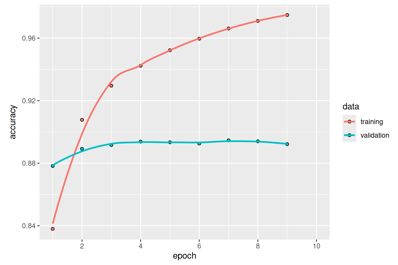

Training and validation metrics for our bag-of-words model.

You can see that validation performance levels off rather than significantly declining; our model is so simple that it cannot really overfit. Let’s try evaluating it on our test set.

Listing 14.14: Evaluating the bag-of-words regression model.

test_result <- evaluate(model, bag_of_words_test_ds)
test_result$accuracy

[1] 0.88692

We can correctly predict the sentiment of a review 88% of the time with a training job light enough that it could run efficiently on a single CPU.

It is worth noting our choice of word tokenization in this example. The reason to avoid character-level tokenization here is pretty obvious: a “bag” of all characters in a movie review will tell us very little about its content. Subword tokenization with a large enough vocabulary would be a good choice, but there is little need for it here. Because the model we are training is so small, it’s convenient to use a vocabulary that is quick to train and have our weights correspond to actual English words.

Preprocessing text efficiently

In all applied machine learning, the speed and efficiency of preprocessing are important concerns. A faster program is always desirable, but this becomes more urgent when the cost of accelerators (GPUs and TPUs) is so high. You want to avoid letting expensive GPUs idle while you preprocess your input!

Text preprocessing is unique because it must always run on a CPU. GPUs strictly handle numeric inputs, so all tokenization must happen before your GPU’s train step. One option is to precompute your tokenized input—tokenization does not depend on model weights, so you could tokenize all input text files and resave them as integer sequences before starting training. However, this is not always practical. Tokenizing text on the fly allows for more rapid experimentation. If you are running inference on an unseen example, there is no way to precompute the tokenized input; you need to tokenize and run a forward pass in rapid succession.

The name of the game when preprocessing text input on the fly is to be “fast enough.” You want to ensure that your expensive GPUs always have a new batch of preprocessed data to ingest. If you do that, the GPU is the bottleneck, and there is nothing to gain by improving your tokenization speed.

You saw tf.data/tfdatasets in previous chapters, and an important reason to use it is that the library is designed to avoid the CPU becoming a bottleneck for a GPU or TPU. We use it throughout this chapter—text_dataset_from_directory() will load a tf.data.Dataset, and dataset_map() will transform our input data, for example by applying a TextVectorization layer. tf.data works by running text preprocessing in parallel on multiple CPU cores, which is generally sufficient to avoid bottlenecking accelerators during a training run.

It is important to note that the code in this chapter is still multi-backend (in fact, we generated the outputs for this chapter using JAX). You can use tf.data with PyTorch, JAX, or TensorFlow itself—Keras will automatically convert input Tensors to the correct format for a given backend.

14.4.2 Training a bigram model

Of course, you can intuitively guess that discarding all word order is very reductive because even atomic concepts can be expressed via multiple words: the term “United States” conveys a concept that is quite distinct from the meaning of the words “states” and “united” taken separately. A movie that is “not bad” and a movie that is “bad” should probably get different sentiment scores.

Therefore, it is usually a good idea to inject some knowledge of local word ordering into a model, even for these simple set-based models we are currently building. One easy way to do that is to consider bigrams: two tokens that appear consecutively in the input text. Given our example “this movie made me cry”, {"this", "movie", "made", "me", "cry"} is the set of all word unigrams in the input, and {"this movie", "movie made", "made me", "me cry"} is the set of all bigrams. The bag-of-words model we just trained could equivalently be called a unigram model, and the term n-gram refers to an ordered sequence of n tokens for any n.

To add bigrams to our model, we want to consider the frequency of all bigrams while building our vocabulary. We can do this in two ways: by creating a vocabulary of only bigrams or by allowing both bigrams and unigrams to compete for space in the same vocabulary. For the latter case, the term "United States" will be included in our vocabulary before "ventriloquism" if it occurs more frequently in the input text.

Again, we could build this by extending our WordTokenizer from earlier in the chapter, but there is no need. TextVectorization provides this out of the box. We will train a slightly larger vocabulary to account for the presence of bigrams, adapt() a new vocabulary, and multi-hot encode output vectors including bigrams.

Listing 14.15: Applying a bigram encoding to the IMDb reviews.

max_tokens <- 30000
text_vectorization <- layer_text_vectorization(
  max_tokens = max_tokens,
1  split = "whitespace",
  output_mode = "multi_hot",
2  ngrams = 2,
)
adapt(text_vectorization, train_ds_no_labels)

bigram_train_ds <- train_ds |>
  dataset_map(\(x, y) tuple(text_vectorization(x), y),
              num_parallel_calls = 8)
bigram_val_ds <- val_ds |>
  dataset_map(\(x, y) tuple(text_vectorization(x), y),
              num_parallel_calls = 8)
bigram_test_ds <- test_ds |>
  dataset_map(\(x, y) tuple(text_vectorization(x), y),
              num_parallel_calls = 8)

1: Learns a word-level vocabulary.
2: Considers all unigrams and bigrams.

Let’s examine a batch of our preprocessed input again:

.[inputs, targets] <- bigram_train_ds |>
  as_iterator() |> iter_next()
str(inputs)

<tf.Tensor: shape=(32, 30000), dtype=int64, numpy=…>

str(targets)

<tf.Tensor: shape=(32), dtype=int32, numpy=…>

If we look at a small subsection of our vocabulary, we can see both unigram and bigram terms:

get_vocabulary(text_vectorization)[100:108]

[1] "first"  "how"    "most"   "him"    "dont"   "it was" "then"   "made"  
[9] "one of"

With our new encoding for our input data, we can train a linear model unaltered from before.

Listing 14.16: Training the bigram regression model.

model <- build_linear_classifier(max_tokens, "bigram_classifier")
model |> fit(
  bigram_train_ds,
  validation_data = bigram_val_ds,
  epochs = 10,
  callbacks = early_stopping
)

This model will be slightly larger than our bag-of-words models (30,001 parameters instead of 20,001 parameters), but it still trains in about the same amount of time. How did it do?

Listing 14.17: Evaluating the bigram regression model.

result <- evaluate(model, bigram_test_ds)
result$accuracy

[1] 0.90176

We’re now getting 90% test accuracy: a noticeable improvement!

We could improve this number even further by considering trigrams (triplets of words), although beyond trigrams, the problem quickly becomes intractable. The space of possible 4-grams of words in the English language is immense, and the problem grows exponentially as sequences get longer and longer. We would need an immense vocabulary to provide decent coverage of 4-grams, and our model would lose its ability to generalize, simply memorizing entire snippets of sentences with weights attached. To robustly consider longer-ordered text sequences, we will need more advanced modeling techniques.

14.5 Sequence models

View on GitHub Run on Colab

Our last two models indicated that sequence information is important. We improved a basic linear model by adding features with some info on local word order.

However, this was done by manually engineering input features, and you can see how the approach will only scale up to a local ordering of just a few words. As is often the case in deep learning, rather than attempting to build these features ourselves, we should expose the model to the raw word sequence and let it directly learn positional dependencies between tokens.

Models that ingest a complete token sequence are called, simply enough, sequence models. We have a few choices for architecture here. We can build an RNN model as we just did for timeseries modeling. We can build a 1D convnet, similar to our image processing models, but convolving filters over a single sequence dimension. And as we will dig into in the next chapter, we can build a Transformer.

Before taking on any of these approaches, we must preprocess our inputs into ordered sequences. We want an integer sequence of token IDs, as we saw in the tokenization portion of this chapter, but with one additional wrinkle to handle. When we run computations on a batch of inputs, we want all inputs to be rectangular so all calculations can be effectively parallelized across the batch on a GPU. However, tokenized inputs will almost always have varying lengths. IMDb movie reviews range from just a few sentences to multiple paragraphs, with varying word counts.

To accommodate this fact, we can truncate our input sequences or “pad” them with another special token "[PAD]", similar to the "[UNK]" token we used earlier. For example, suppose we have two input sentences and a desired length of eight:

"the quick brown fox jumped over the lazy dog"
"the slow brown badger"

We can tokenize to the integer IDs for the following tokens:

c("the", "quick", "brown", "fox", "jumped", "over", "the", "lazy")
c("the", "slow", "brown", "badger", "[PAD]", "[PAD]", "[PAD]", "[PAD]")

This will allow our batch computation to proceed much faster, although we will need to be careful with our padding tokens to ensure that they do not affect the quality of our model predictions.

To keep a manageable input size, we can truncate our IMDb reviews after the first 600 words. This is a reasonable choice, because the average review length is 233 words, and only 5% of reviews are longer than 600 words. Once again, we can use the TextVectorization layer, which has an option for padding or truncating inputs and includes a "[PAD]" at index zero of the learned vocabulary.

Listing 14.18: Padding IMDb reviews to a fixed sequence length.

max_length <- 600
max_tokens <- 30000
text_vectorization <- layer_text_vectorization(
  max_tokens = max_tokens,
1  split = "whitespace",
2  output_mode = "int",
3  output_sequence_length = max_length
)
text_vectorization |> adapt(train_ds_no_labels)

sequence_train_ds <- train_ds |>
  dataset_map(\(x, y) tuple(text_vectorization(x), y),
              num_parallel_calls = 8)
sequence_val_ds <- val_ds |>
  dataset_map(\(x, y) tuple(text_vectorization(x), y),
              num_parallel_calls = 8)
sequence_test_ds <- test_ds |>
  dataset_map(\(x, y) tuple(text_vectorization(x), y),
              num_parallel_calls = 8)

1: Learns a word-level vocabulary.
2: Outputs an integer sequence of token IDs.
3: Pads and truncates to 600 tokens.

Let’s take a look at a single input batch:

.[x, y] <- sequence_test_ds |> as_array_iterator() |> iter_next()
str(x)

 num [1:32, 1:600] 142 10 274 50 11 10 10 117 197 255 ...

tail(x, c(5, 5))

      [,596] [,597] [,598] [,599] [,600]
[28,]      0      0      0      0      0
[29,]      0      0      0      0      0
[30,]      0      0      0      0      0
[31,]      0      0      0      0      0
[32,]     52   6348      4     31    212

Each batch has the shape (batch_size, sequence_length) after preprocessing, and almost all training samples have a number of 0s for padding at the end.

14.5.1 Training a recurrent model

Let’s try training an LSTM. As we saw in the previous chapter, LSTMs can work efficiently with sequence data. Before we can apply it, we still need to map our token ID integers into floating-point data ingestible by a Dense layer.

The most straightforward approach is to one-hot our input IDs, similar to the multi-hot encoding we did for an entire sequence. Each token will become a long vector with all 0s and a single 1 at the index of the token in our vocabulary. Let’s build a layer to one-hot encode our input sequence.

We can use the op_one_hot() operation directly on a tensor with the Function API, as if it was a (stateless) layer. We can build this layer directly into a model, and use a bidirectional LSTM to allow information to propagate both forward and backward along the token sequence. Later, when we look at generation, we will see the need for unidirectional sequence models (where a token state only depends on the token state before it). For classification tasks, a bidirectional LSTM is a good fit. Let’s build our model.

Listing 14.19: Building an LSTM sequence model.

hidden_dim <- 64
inputs <- keras_input(shape = c(max_length), dtype = "int32")
outputs <- inputs |>
  op_one_hot(num_classes = max_tokens, zero_indexed = TRUE) |>
  layer_bidirectional(layer_lstm(units = hidden_dim)) |>
  layer_dropout(0.5) |>
  layer_dense(1, activation = "sigmoid")

model <- keras_model(inputs, outputs, name = "lstm_with_one_hot")
model |> compile(optimizer = "adam",
                 loss = "binary_crossentropy",
                 metrics = c("accuracy"))

We can take a look at our model summary to get a sense of our parameter count:

model

Model: "lstm_with_one_hot"
┏━━━━━━━━━━━━━━━━━━━━━━━━━━━━━━━━━┳━━━━━━━━━━━━━━━━━━━━━━━━┳━━━━━━━━━━━━━━━┓
┃ Layer (type)                    ┃ Output Shape           ┃       Param # ┃
┡━━━━━━━━━━━━━━━━━━━━━━━━━━━━━━━━━╇━━━━━━━━━━━━━━━━━━━━━━━━╇━━━━━━━━━━━━━━━┩
│ input_layer_2 (InputLayer)      │ (None, 600)            │             0 │
├─────────────────────────────────┼────────────────────────┼───────────────┤
│ one_hot (OneHot)                │ (None, 600, 30000)     │             0 │
├─────────────────────────────────┼────────────────────────┼───────────────┤
│ bidirectional (Bidirectional)   │ (None, 128)            │    15,393,280 │
├─────────────────────────────────┼────────────────────────┼───────────────┤
│ dropout (Dropout)               │ (None, 128)            │             0 │
├─────────────────────────────────┼────────────────────────┼───────────────┤
│ dense_2 (Dense)                 │ (None, 1)              │           129 │
└─────────────────────────────────┴────────────────────────┴───────────────┘
 Total params: 15,393,409 (58.72 MB)
 Trainable params: 15,393,409 (58.72 MB)
 Non-trainable params: 0 (0.00 B)

This is quite the step up in size from the unigram and bigram models. At about 15 million parameters, this is one of the larger models we have trained in the book so far, with only a single LSTM layer. Let’s try training the model.

Listing 14.20: Training the LSTM sequence model.

model |> fit(
  sequence_train_ds,
  validation_data = sequence_val_ds,
  epochs = 10,
  callbacks = c(early_stopping)
)

How does it perform?

Listing 14.21: Evaluating the LSTM sequence model.

evaluate(model, sequence_test_ds)$accuracy

[1] 0.6964

This model works, but it trains very slowly, especially compared to the lightweight model of the previous section. That’s because our inputs are large: each input sample is encoded as a matrix of size (600, 30000) (600 words per sample, 30,000 possible words). That is 18,000,000 floating-point numbers for a single movie review! Our bidirectional LSTM has a lot of work to do. In addition to being slow, the model reaches only 70% test accuracy—it doesn’t perform nearly as well as our very fast set-based models.

Clearly, using one-hot encoding to turn words into vectors, which was the simplest thing we could do, wasn’t a great idea. There’s a better way: word embeddings.

14.5.2 Understanding word embeddings

When we encode something via one-hot encoding, we’re making a feature engineering decision. We’re injecting into the model a fundamental assumption about the structure of our feature space. That assumption is that the different tokens we’re encoding are all independent from each other: indeed, one-hot vectors are all orthogonal to one another. In the case of words, that assumption is clearly wrong. Words form a structured space: they share information with each other. The words “movie” and “film” are interchangeable in most sentences, so the vector that represents “movie” should not be orthogonal to the vector that represents “film”—they should be the same vector, or close enough.

To get more abstract, the geometric relationship between two-word vectors should reflect the semantic relationship between these words. For instance, in a reasonable word vector space, we would expect synonyms to be embedded into similar word vectors, and in general, we would expect the geometric distance (such as the cosine distance or L2 distance) between any two-word vectors to relate to the “semantic distance” between the associated words. Words that mean different things should lie far away from each other, whereas related words should be closer. Word embeddings are vector representations of words that achieve precisely this: they map human language into a structured geometric space.

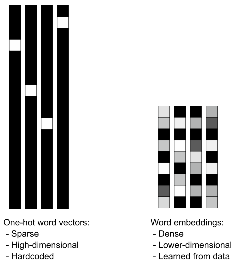
Whereas the vectors obtained through one-hot encoding are binary, sparse (mostly made of zeros), and very high-dimensional (the same dimensionality as the number of words in the vocabulary), word embeddings are low-dimensional floating-point vectors (that is, dense vectors, as opposed to sparse vectors); see figure 14.3. It’s common to see word embeddings that are 256-dimensional, 512-dimensional, or 1,024-dimensional when dealing with very large vocabularies. On the other hand, one-hot encoding words generally leads to vectors that are 30,000-dimensional in the case of our current vocabulary. So, word embeddings pack more information into far fewer dimensions.

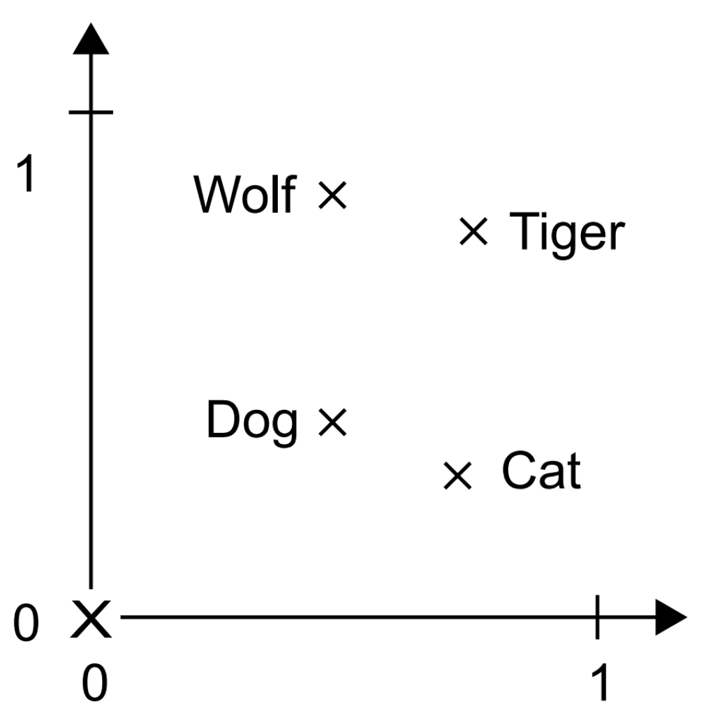
Word representations obtained from one-hot encoding or hashing are sparse, high-dimensional, and hardcoded. Word embeddings are dense, relatively low-dimensional, and learned from data.

Besides being dense representations, word embeddings are also structured representations, and their structure is learned from data. Similar words get embedded in close locations, and further, specific directions in the embedding space are meaningful. To make this clearer, let’s look at a concrete example. In figure 14.4, four words are embedded on a 2D plane: “cat,” “dog,” “wolf,” and “tiger.” With the vector representations we chose here, some semantic relationships between these words can be encoded as geometric transformations. For instance, the same vector allows us to go from “cat” to “tiger” and from “dog” to “wolf”: this vector could be interpreted as the “from pet to wild animal” vector. Similarly, another vector lets us go from “dog” to “cat” and from “wolf” to “tiger,” which could be interpreted as a “from canine to feline” vector.

In real-world word-embedding spaces, typical examples of meaningful geometric transformations are “gender” vectors and “plural” vectors. For instance, by adding a “female” vector to the vector “king,” we obtain the vector “queen.” By adding a “plural” vector, we obtain “kings.” Word-embedding spaces typically feature thousands of such interpretable and potentially useful vectors. Let’s look at how to use such an embedding space in practice.

14.5.3 Using a word embedding

Is there an ideal word-embedding space that perfectly maps human language and can be used for any NLP task? Possibly, but we have yet to compute anything of the sort. Also, there is no single human language we could attempt to map—there are many different languages, and they aren’t isomorphic to one another because a language is the reflection of a specific culture and a particular context. More pragmatically, what makes a good word-embedding space depends heavily on the task: the perfect word-embedding space for an English-language movie review sentiment-analysis model may look different from the ideal embedding space for an English-language legal document classification model because the importance of certain semantic relationships varies from task to task.

It’s thus reasonable to learn a new embedding space with every new task. Fortunately, backpropagation makes this easy, and Keras makes it even easier. It’s about learning the weights of the Keras Embedding layer.

The Embedding layer is best understood as a dictionary that maps integer indices (which stand for specific words) to dense vectors. It takes integers as input, looks them up in an internal dictionary, and returns the associated vectors. It’s effectively a dictionary lookup (see figure 14.5).

An Embedding layer acts as a dictionary mapping ints to floating-point vectors. — An `Embedding` layer acts as a dictionary mapping ints to floating-point vectors.

The Embedding layer takes as input a rank-2 tensor with shape (batch_size, sequence_length), where each entry is a sequence of integers. The layer returns a floating-point tensor of shape (batch_size, sequence_length, embedding_size).

When we instantiate an Embedding layer, its weights (its internal dictionary of token vectors) are initially random, just as with any other layer. During training, these word vectors are gradually adjusted via backpropagation, structuring the space into something the downstream model can exploit. Once fully trained, the embedding space will show a lot of structure—a kind of structure specialized for the specific problem for which we’re training our model.

Let’s build a model with an Embedding layer and benchmark it on our task.

Listing 14.22: Building an LSTM sequence model with an Embedding layer.

hidden_dim <- 64L
inputs <- keras_input(shape = c(max_length), dtype = "int32")
outputs <- inputs |>
  layer_embedding(input_dim = max_tokens,
                  output_dim = hidden_dim,
                  mask_zero = TRUE) |>
  layer_bidirectional(layer_lstm(units = hidden_dim)) |>
  layer_dropout(0.5) |>
  layer_dense(1, activation = "sigmoid")

model <- keras_model(inputs, outputs, name = "lstm_with_embedding")
model |> compile(optimizer = "adam",
                 loss = "binary_crossentropy",
                 metrics = "accuracy")

The first two arguments to the Embedding layer are fairly straightforward. input_dim sets the total range of possible values for the integer inputs to the layer—that is, how many possible keys are in our dictionary lookup. output_dim sets the dimensionality of the output vector we look up—that is, the dimensionality of our structured vector space for words.

The third argument, mask_zero = TRUE, is a little more subtle. This argument tells Keras which inputs in our sequence are "[PAD]" tokens so we can mask these entries later in the model.

Remember that when preprocessing our sequence input, we might add a lot of padding tokens to our original input, so a token sequence might look like this:

c("the", "movie", "was", "awful", "[PAD]", "[PAD]", "[PAD]", "[PAD]")

All of those padding tokens will be first embedded and then fed into the LSTM layer. This means the last representation we receive from the LSTM cell might contain the results of processing the "[PAD]" token representation over and over recurrently. We are not very interested in the learned LSTM representation for the last "[PAD]" token in the previous sequence. Instead, we are interested in the representation of "awful", the last non-padding token. Or, put equivalently, we want to mask all of the "[PAD]" tokens so that they do not affect our final output prediction.

mask_zero=TRUE is simply a shorthand to easily do such masking in Keras with the Embedding layer. Keras will mark all elements in our sequence that initially contained a zero value, where zero is assumed to be the token ID for the "[PAD]" token. This mask will be used internally by the LSTM layer. Instead of outputting the last learned representation for the whole sequence, it will output the last non-masked representation.

This form of masking is implicit and easy to use, but we can always be explicit about which items in a sequence we would like to mask if the need arises. The LSTM layer takes an optional mask call argument, for explicit or custom masking.

Before we train this new model, let’s take a look at the model summary:

model

Model: "lstm_with_embedding"
┏━━━━━━━━━━━━━━━━━━━━━┳━━━━━━━━━━━━━━━━━━━┳━━━━━━━━━━━━┳━━━━━━━━━━━━━━━━━━━┓
┃ Layer (type)        ┃ Output Shape      ┃    Param # ┃ Connected to      ┃
┡━━━━━━━━━━━━━━━━━━━━━╇━━━━━━━━━━━━━━━━━━━╇━━━━━━━━━━━━╇━━━━━━━━━━━━━━━━━━━┩
│ input_layer_3       │ (None, 600)       │          0 │ -                 │
│ (InputLayer)        │                   │            │                   │
├─────────────────────┼───────────────────┼────────────┼───────────────────┤
│ embedding           │ (None, 600, 64)   │  1,920,000 │ input_layer_3[0]… │
│ (Embedding)         │                   │            │                   │
├─────────────────────┼───────────────────┼────────────┼───────────────────┤
│ not_equal           │ (None, 600)       │          0 │ input_layer_3[0]… │
│ (NotEqual)          │                   │            │                   │
├─────────────────────┼───────────────────┼────────────┼───────────────────┤
│ bidirectional_1     │ (None, 128)       │     66,048 │ embedding[0][0],  │
│ (Bidirectional)     │                   │            │ not_equal[0][0]   │
├─────────────────────┼───────────────────┼────────────┼───────────────────┤
│ dropout_1 (Dropout) │ (None, 128)       │          0 │ bidirectional_1[… │
├─────────────────────┼───────────────────┼────────────┼───────────────────┤
│ dense_3 (Dense)     │ (None, 1)         │        129 │ dropout_1[0][0]   │
└─────────────────────┴───────────────────┴────────────┴───────────────────┘
 Total params: 1,986,177 (7.58 MB)
 Trainable params: 1,986,177 (7.58 MB)
 Non-trainable params: 0 (0.00 B)

We have reduced the number of parameters for our one-hot-encoded LSTM model from 15 million to 2 million. Let’s train and evaluate the model.

Listing 14.23: Training and evaluating the LSTM with an Embedding layer.

model |> fit(
  sequence_train_ds,
  validation_data = sequence_val_ds,
  epochs = 10,
  callbacks = early_stopping
)
result <- evaluate(model, sequence_test_ds)
result$accuracy

[1] 0.8602

With the embedding, we have reduced both our training time and model size by an order of magnitude. A learned embedding is clearly far more efficient than one-hot encoding our input.

However, the LSTM’s overall performance did not change. Accuracy was stubbornly around 86%, still a far cry from the bag-of-words and bigram models. Does this mean that a “structured embedding space” for input tokens is not that practically useful? Or is it not useful for text classification tasks?

Quite the contrary: a well-trained token embedding space can dramatically improve the practical performance ceiling of a model like this. The problem in this particular case is with our training setup. We lack enough data in our 20,000 review examples to effectively train a good word embedding. By the end of our 10 training epochs, our training set accuracy has cracked 99%. Our model has begun to overfit and memorize our input, and it turns out it is doing so well before we have learned an optimal set of word embeddings for the task at hand.

For cases like this, we can turn to pretraining. Rather than training our word embedding jointly with the classification task, we can train it separately, on more data, without the need for positive and negative review labels. Let’s take a look.

Augmenting text data

After seeing the importance of data augmentation for computer vision problems, you might wonder if you can do the same for text. The short answer is yes, you can, although it is not nearly as effective in the text domain.

Basic text augmentation techniques look for edits we can make to input text that might help make our model more robust. For example, we might randomly delete or swap the position of words in a sentence, so the sentence “The rain in Spain falls mainly on the plain” becomes “The rain Spain falls plain on the mainly.” Training a model on such edited inputs can make it robust to typos and grammar mistakes.

However, this example also concisely shows the big pitfall with text augmentation: it is easy to alter the meaning of an input example unintentionally. Unlike image data, where we can crop, rotate, and adjust color levels on a picture of a cat and still have a recognizable cat on the other end, language is order-dependent and highly sensitive to tiny changes. A sentence with two words swapped might mean the opposite of the input sentence. Some augmentation techniques seek to solve this by replacing words from a table of known synonyms, but this, too, can be brittle if we choose the incorrect meaning of a word. These problems have kept text augmentation from being widespread in practice. It is usually a better idea to seek more text examples than to sink time into text augmentation techniques.

Generative models, which we will see in the coming chapters, are beginning to offer a new form of text augmentation that can alleviate these pain points. By generating outputs from a model that has learned how to produce consistent and coherent text, we can create completely unseen inputs that plausibly resemble our input data. This poses its own challenges but opens up a new frontier for text augmentation on problems where data is particularly sparse and challenging to collect.

14.5.4 Pretraining a word embedding

The last decade of rapid advancement in NLP has coincided with the rise of pretraining as the dominant approach for text modeling problems. Once we move past simple set-based regression models to sequence models with millions or even billions of parameters, text models become incredibly data-hungry. We are usually limited by our ability to find labeled examples for a particular problem in the text domain.

The idea is to devise an unsupervised task to train model parameters that do not need labeled data. Pretraining data can be text in a similar domain to our final task, or even arbitrary text in the languages we are interested in working with. Pretraining allows us to learn general patterns in language, effectively priming our model before we specialize it to the final task we are interested in.

Word embeddings were one of the first big successes with text pretraining, and we will show how to pretrain a word embedding in this section. Remember the unsup/ directory we ignored in our IMDb dataset preparation? It contains another 25,000 reviews—the same size as our training data. We will combine all our training data and show how to pretrain the parameters of an Embedding layer with an unsupervised task.

One of the most straightforward setups for training a word embedding is called the Continuous Bag of Words (CBOW) model². The idea is to slide a window over all the text in a dataset, where we continuously attempt to guess a missing word based on the words that appear to its direct right and left (figure 14.6). For example, if our “bag” of surrounding words contained the words “sail,” “wave,” and “mast,” we might guess that the middle word is “boat” or “ocean.”

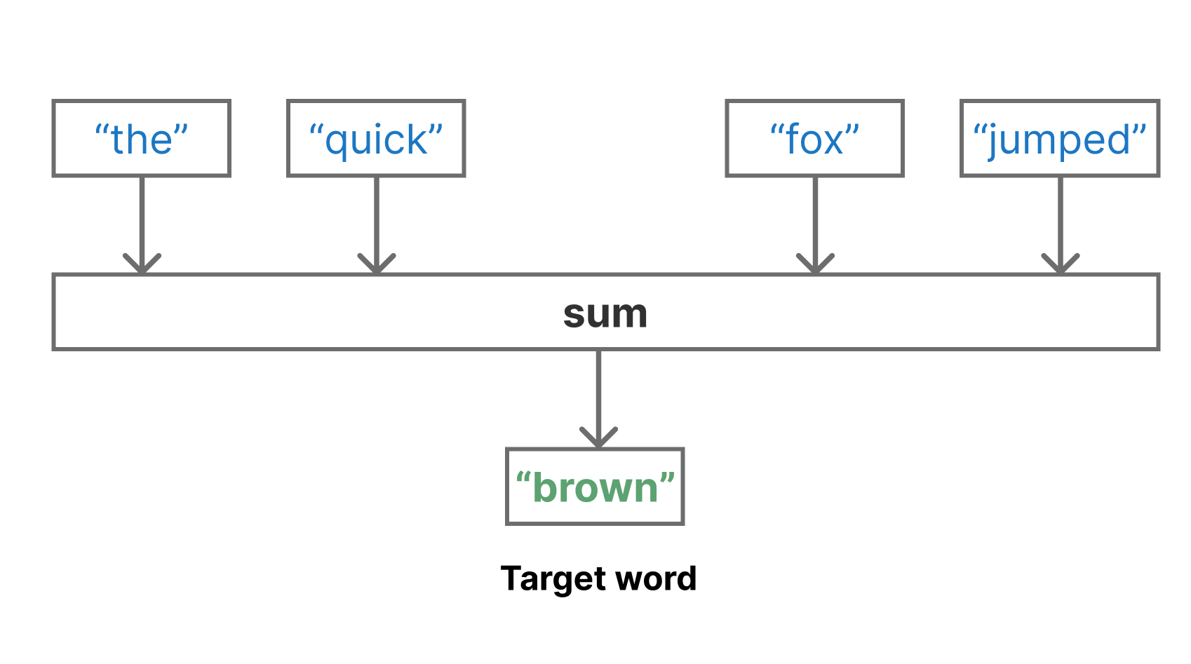
The Continuous Bag of Words predicts a word based on its surrounding context with a shallow neural network.

In our particular IMDb classification problem, we are interested in “priming” the word embedding of the LSTM model we just trained. We can reuse the TextVectorization vocabulary we computed earlier. All we are trying to do here is to learn a good 64-dimensional vector for each word in this vocabulary.

We can create a new TextVectorization layer with the same vocabulary that does not truncate or pad input. We will preprocess the output tokens of this layer by sliding a context window across our text.

Listing 14.24: Removing padding from our TextVectorization preprocessing layer.

imdb_vocabulary <- text_vectorization |> get_vocabulary()
tokenize_no_padding <- layer_text_vectorization(
  vocabulary = imdb_vocabulary,
  split = "whitespace",
  output_mode = "int"
)

To preprocess our data, we will slide a window across our training data, creating “bags” of nine consecutive tokens. Then, we’ll use the middle word as our label and the remaining eight words as an unordered context to predict our label. To do this, we will again use tf.data to preprocess our inputs, although this choice does not limit the backend we use for actual model training.

Listing 14.25: Preprocessing our IMDb data for pretraining a CBOW model.

1context_size <- 4L
2window_size <- context_size + 1L + context_size

window_data <- function(token_ids) {
  windows <- tf$signal$frame(
    token_ids,
    frame_length = window_size,
    frame_step = 1L
  )
  tensor_slices_dataset(windows)
}

split_label <- function(window) {
  .[left, label, right] <-
    tf$split(window, c(context_size, 1L, context_size))
  bag <- tf$concat(tuple(left, right), axis = 0L)
  tuple(bag, label)
}

3dataset <- text_dataset_from_directory("aclImdb/train", batch_size = NULL)

dataset <- dataset |>
4  dataset_map(\(x, y) x, num_parallel_calls = 8) |>
5  dataset_map(tokenize_no_padding, num_parallel_calls = 8) |>
6  dataset_interleave(window_data) |>
7  dataset_map(split_label, num_parallel_calls = 8)

1: Words to the left or right of the label
2: Total window size
3: Uses all training data, including the unsup/ directory.
4: Drops the label
5: Tokenizes
6: Creates context windows
7: Splits the middle word into a label

Found 70000 files belonging to 3 classes.

After preprocessing, we have eight integer token IDs as context, paired with a single token ID label.

The model we train with this data is exceedingly simple. We will use an Embedding layer to embed all context tokens and a GlobalAveragePooling1D to compute the average embedding of our “bag” of context tokens. Then we’ll use that average embedding to predict the value of our middle label token.

That’s it! By repeatedly refining our embedding space so that we are good at predicting a word based on nearby word embeddings, we can learn a rich embedding of tokens used in movie reviews.

Listing 14.26: Building a CBOW model.

hidden_dim <- 64

cbow_embedding <- layer_embedding(
  input_dim = max_tokens,
  output_dim = hidden_dim
)

inputs <- keras_input(shape = c(2 * context_size))

outputs <- inputs |>
  cbow_embedding() |>
  layer_global_average_pooling_1d() |>
  layer_dense(max_tokens, activation = "softmax")

cbow_model <- keras_model(inputs, outputs)
cbow_model |> compile(
  optimizer = "adam",
  loss = "sparse_categorical_crossentropy",
  metrics = "sparse_categorical_accuracy"
)

cbow_model

Model: "functional"
┏━━━━━━━━━━━━━━━━━━━━━━━━━━━━━━━━━┳━━━━━━━━━━━━━━━━━━━━━━━━┳━━━━━━━━━━━━━━━┓
┃ Layer (type)                    ┃ Output Shape           ┃       Param # ┃
┡━━━━━━━━━━━━━━━━━━━━━━━━━━━━━━━━━╇━━━━━━━━━━━━━━━━━━━━━━━━╇━━━━━━━━━━━━━━━┩
│ input_layer_4 (InputLayer)      │ (None, 8)              │             0 │
├─────────────────────────────────┼────────────────────────┼───────────────┤
│ embedding_1 (Embedding)         │ (None, 8, 64)          │     1,920,000 │
├─────────────────────────────────┼────────────────────────┼───────────────┤
│ global_average_pooling1d        │ (None, 64)             │             0 │
│ (GlobalAveragePooling1D)        │                        │               │
├─────────────────────────────────┼────────────────────────┼───────────────┤
│ dense_4 (Dense)                 │ (None, 30000)          │     1,950,000 │
└─────────────────────────────────┴────────────────────────┴───────────────┘
 Total params: 3,870,000 (14.76 MB)
 Trainable params: 3,870,000 (14.76 MB)
 Non-trainable params: 0 (0.00 B)

Because our model is so simple, we can use a large batch size to speed up training without worrying about memory constraints. We will also call dataset_cache() on this batched dataset so that we store the entire preprocessed dataset in memory rather than recomputing it each epoch. This is because, for this very simple model, we are bottlenecked on preprocessing rather than training. That is, it is slower to tokenize our text and compute sliding windows on the CPU than to update our model parameters on the GPU.

In such cases, saving your preprocessed outputs in memory or on disk is usually a good idea. You will notice how later epochs are more than three times faster than the first. This is thanks to the cache of preprocessed training data.

Listing 14.27: Training the CBOW model.

dataset <- dataset |> dataset_batch(1024) |> dataset_cache()
cbow_model |> fit(dataset, epochs = 4)

At the end of training, we are able to guess the middle word around 12% of the time based solely on the neighboring eight words. This may not sound like a great result, but given that we have 30,000 words to guess from each time, this is actually a reasonable accuracy score. Let’s use this word embedding to improve the performance of our LSTM model.

14.5.5 Using the pretrained embedding for classification

Now that we have trained a new word embedding, applying it to our LSTM model is simple. First, we create the model precisely as we did before.

Listing 14.28: Building another LSTM sequence model with an Embedding layer.

inputs <- keras_input(shape = c(max_length))
lstm_embedding <- layer_embedding(
  input_dim = max_tokens,
  output_dim = hidden_dim,
  mask_zero = TRUE
)
outputs <- inputs |>
  lstm_embedding() |>
  layer_bidirectional(layer_lstm(units = hidden_dim)) |>
  layer_dropout(0.5) |>
  layer_dense(1, activation = "sigmoid")

model <- keras_model(inputs, outputs, name = "lstm_with_cbow")

Then, we apply our embedding weights from the CBOW embedding layer to the LSTM embedding layer. This effectively acts as a new and better initializer for the roughly 2 million embedding parameters in the LSTM model.

Listing 14.29: Reusing the CBOW embedding to prime the LSTM model.

lstm_embedding$embeddings$assign(cbow_embedding$embeddings)

With that, we can compile and train our LSTM model as normal.

Listing 14.30: Training the LSTM model with a pretrained embedding.

model |> compile(
  optimizer = "adam",
  loss = "binary_crossentropy",
  metrics = "accuracy"
)
model |> fit(
  sequence_train_ds,
  validation_data = sequence_val_ds,
  epochs = 10,
  callbacks = c(early_stopping)
)

Let’s evaluate our LSTM model.

Listing 14.31: Evaluating the LSTM model with a pretrained embedding.

result <- evaluate(model, sequence_test_ds)
result$accuracy

[1] 0.89139

With the pretrained embedding weights, we have boosted our LSTM performance to roughly the same level as our set-based models. We do slightly better than the unigram model and slightly worse than the bigram model.

This may seem like a bit of a letdown after all the work we put in. Is learning on the entire sequence, with order information, just a bad idea? The problem is that we are still data-constrained for our final LSTM model. The model is expressive and powerful enough that with enough movie reviews, we would easily outperform set-based approaches, but we need a lot more training on ordered data before our model’s performance ceiling is reached.

This is an easily solvable problem with enough compute resources. In the next chapter, we will cover the Transformer model. The model is slightly better at learning dependencies across longer token sequences, but, most critically, these models are often trained on large amounts of English text, including all word order information. This allows the model to learn, roughly speaking, a statistical form of the grammatical patterns that govern language. These types of statistical patterns around word order are precisely why our current LSTM model is too data-constrained to learn effectively.

However, as we move on to large, more advanced models that will push the limits of text-classification performance, it is worth pointing out that simple set-based regression approaches like our bigram model give you a lot of “bang for your buck.” Set-based models are lightning-fast and can contain just a few thousand parameters, a far cry from the billion-parameter large language models that dominate the news today. If you are working in an environment where compute is limited and you can sacrifice some accuracy, set-based models can often be the most cost-effective approach.

14.6 Summary

All text modeling problems involve a preprocessing step where text is broken up and transformed to integer data, called tokenization.
Tokenization can be divided into three steps: standardization, splitting, and indexing. Standardization normalizes text, splitting breaks text up into tokens, and indexing assigns each token a unique integer ID.
There are three main types of tokenization: character, word, and subword tokenization. With an expressive enough model and enough training data, subword tokenization is usually the most effective.
NLP models differ primarily in handling the order of input tokens:
- Set models discard most order information and learn simple and fast models based solely on the presence or absence of tokens in the input. Bigram or trigram models consider the presence or absence of two or three consecutive tokens. Set models are incredibly fast to train and deploy.
- Sequence models attempt to learn with the ordered sequence of tokens in the input data. Sequence models need large amounts of data to learn effectively.
An embedding is an efficient way to transform token IDs into a learned latent space. Embeddings can be trained normally with gradient descent.
Pretraining is critical for sequence models as a way to get around the data-hungry nature of these models. During pretraining, an unsupervised task allows models to learn from large amounts of unlabeled text data. The learned parameters can then be transferred to a downstream task.

Phillip Gage, “A New Algorithm for Data Compression”, The C Users Journal Archive (1994), https://dl.acm.org/doi/10.5555/177910.177914.↩︎
Tomas Mikolov et al., “Efficient Estimation of Word Representations in Vector Space”, International Conference on Learning Representations (2013), https://arxiv.org/abs/1301.3781.↩︎