- 1
- Encodes the input into a mean and variance parameter
- 2
- Draws a latent point using a small random epsilon
- 3
- Decodes z back to an image
- 4
- Instantiates the autoencoder model, which maps an input image to its reconstruction
17 Image generation
This chapter covers
- Using variational autoencoders
- Understanding diffusion models
- Using a pretrained text-to-image model
- Exploring the image latent spaces learned by text-to-image models
The most popular and successful application of creative AI today is image generation: learning latent visual spaces and sampling from them to create entirely new pictures, interpolated from real ones: pictures of imaginary people, imaginary places, imaginary cats and dogs, and so on.
17.1 Deep learning for image generation
In this section and the next, we’ll review some high-level concepts pertaining to image generation, alongside implementation details relative to two of the main techniques in this domain: variational autoencoders (VAEs) and diffusion models. Note that the techniques we present here aren’t specific to images—you could develop latent spaces of sound or music using similar models—but in practice, the most interesting results so far have been obtained with pictures, and that’s what we focus on here.
17.1.1 Sampling from latent spaces of images
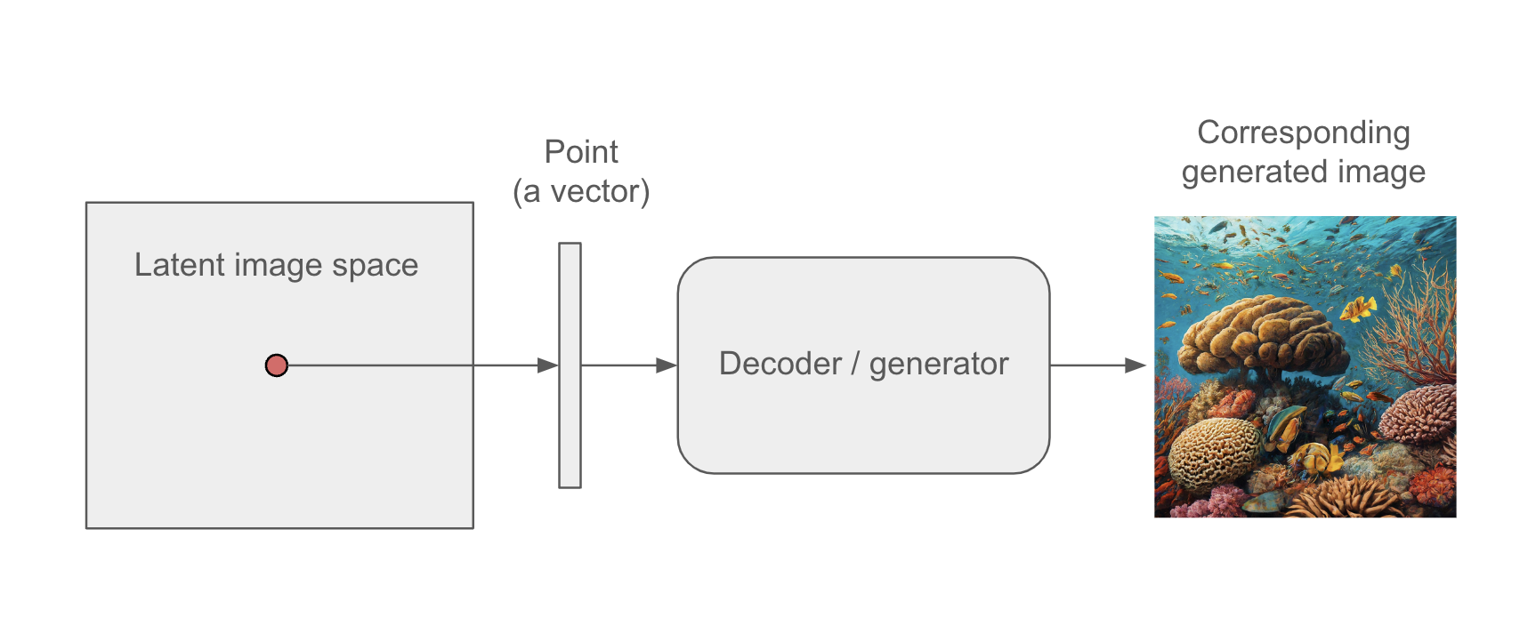
The key idea of image generation is to develop a low-dimensional latent space of representations (which, like everything else in deep learning, is a vector space) where any point can be mapped to a “valid” image: an image that looks like the real thing. The module capable of realizing this mapping, taking as input a latent point and outputting an image (a grid of pixels), is usually called a generator, or sometimes a decoder. Once such a latent space has been learned, you can sample points from it and, by mapping them back to image space, generate images that have never been seen before (see figure 17.1)—the in-betweens of the training images.
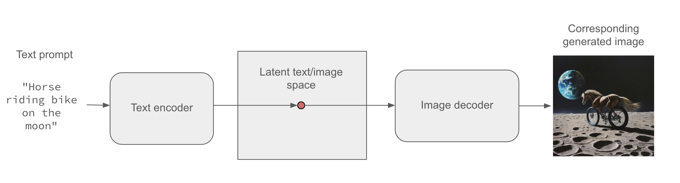
Further, text-conditioning makes it possible to map a space of prompts in natural language to the latent space (see figure 17.2), making it possible to do language-guided image generation: generating pictures that correspond to a text description. This category of models is called text-to-image models.
Interpolating between many training images in the latent space enables such models to generate infinite combinations of visual concepts, including many that no one had explicitly come up with before. A horse riding a bike on the moon? You got it. This makes image generation a powerful brush for creative-minded people to play with.
Of course, there are still challenges to overcome. As with all deep learning models, the latent space doesn’t encode a consistent model of the physical world, so you might occasionally see hands with extra fingers, incoherent lighting, or garbled objects. The coherence of generated images is still an area of active research. In the case of figure 17.2, despite having seen tens of thousands of images of people riding bikes, the model doesn’t understand in a human sense what it means to ride a bike—concepts like pedaling, steering, or maintaining upright balance. That’s why our bike-riding horse is unlikely to be depicted pedaling with its hind legs in a believable manner, the way a human artist would draw it.
There’s a range of different strategies for learning such latent spaces of image representations, each with its own characteristics. The most common types of image generation models are these:
- Diffusion models
- Variational autoencoders (VAEs)
- Generative adversarial networks (GANs)
Previous editions of this book covered GANs, but they have gradually fallen out of fashion in recent years and have been all but replaced by diffusion models. In this edition, we’ll cover both VAEs and diffusion models, and we will skip GANs. In the models we’ll build ourselves, we’ll focus on unconditioned image generation: sampling images from a latent space without text conditioning. However, you will also learn how to use a pretrained text-to-image model and how to explore its latent space.
17.1.2 Variational autoencoders
VAEs, simultaneously discovered by Diederik P. Kingma and Max Welling in December 20131 and Danilo Jimenez Rezende, Shakir Mohamed, and Daan Wierstra in January 20142 are a kind of generative model that’s especially appropriate for the task of image editing via concept vectors. They’re a kind of autoencoder—a type of network that aims to encode an input to a low-dimensional latent space and then decode it back—that mixes ideas from deep learning with Bayesian inference.
VAEs have been around for more than a decade, but they remain relevant to this day and continue to be used in recent research. Although VAEs will never be the first choice for generating high-fidelity images—where diffusion models excel—they remain an important tool in the deep learning toolbox, particularly when interpretability, control over the latent space, and data reconstruction capabilities are crucial. It’s also your first contact with the concept of the autoencoder, which is useful to know about. VAEs beautifully illustrate the core idea behind this class of models.
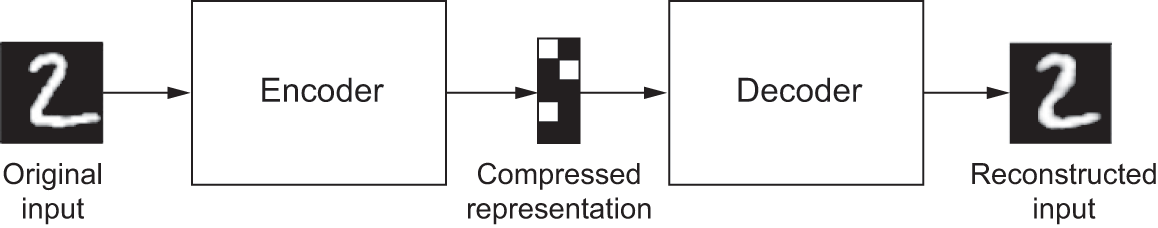
A classical image autoencoder takes an image, maps it to a latent vector space via an encoder module, and then decodes it back to an output with the same dimensions as the original image, via a decoder module (see figure 17.3). It’s then trained by using as target data the same images as the input images, meaning the autoencoder learns to reconstruct the original inputs. By imposing various constraints on the code (the output of the encoder), we can get the autoencoder to learn more or less interesting latent representations of the data. Most commonly, we constrain the code to be low-dimensional and sparse (mostly zeros), in which case the encoder acts as a way to compress the input data into fewer bits of information.
In practice, such classical autoencoders don’t lead to particularly useful or nicely structured latent spaces. They’re not much good at compression, either. For these reasons, they have largely fallen out of fashion. VAEs, however, augment autoencoders with a little statistical magic that forces them to learn continuous, highly structured latent spaces. They have turned out to be a powerful tool for image generation.
A VAE, instead of compressing its input image into a fixed code in the latent space, turns the image into the parameters of a statistical distribution: a mean and a variance. Essentially, this means we’re assuming the input image has been generated by a statistical process and that the randomness of this process should be taken into account during encoding and decoding. The VAE then uses the mean and variance parameters to randomly sample one element of the distribution, and decodes that element back to the original input (see figure 17.4). The stochasticity of this process improves robustness and forces the latent space to encode meaningful representations everywhere: every point sampled in the latent space is decoded to a valid output.
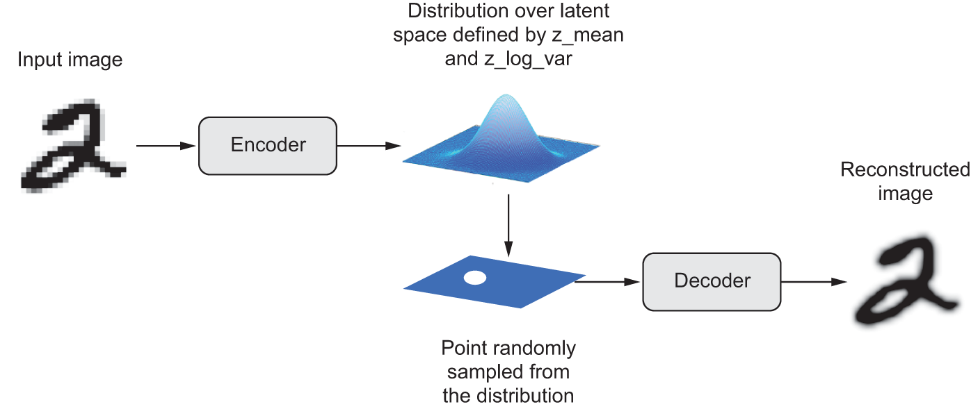
z_mean and z_log_var, which define a probability distribution over the latent space, used to sample a latent point to decode.In technical terms, here’s how a VAE works:
An encoder module turns the input sample
input_imginto two parameters in a latent space of representations,z_meanandz_log_var(log variance).We randomly sample a point
zfrom the latent normal distribution that’s assumed to generate the input image, viaz = z_mean + exp(0.5 * z_log_var) * epsilon, whereepsilonis a random tensor of small values.A decoder module maps this point in the latent space back to the original input image.
Because epsilon is random, the process ensures that every point that’s close to the latent location where we encoded input_img (z_mean) can be decoded to something similar to input_img, thus forcing the latent space to be continuously meaningful. Any two close points in the latent space will decode to highly similar images. Continuity, combined with the low dimensionality of the latent space, forces every direction in the latent space to encode a meaningful axis of variation of the data, making the latent space very structured and thus highly suitable to manipulation via concept vectors.
The parameters of a VAE are trained via two loss functions: a reconstruction loss that forces the decoded samples to match the initial inputs, and a regularization loss that helps learn well-rounded latent distributions and reduces overfitting to the training data. Schematically, the process looks like this:
We can then train the model using the reconstruction loss and the regularization loss. For the regularization loss, we typically use an expression (the Kullback–Leibler divergence) meant to nudge the distribution of the encoder output toward a well-rounded normal distribution centered around 0. This provides the encoder with a sensible assumption about the structure of the latent space it’s modeling.
Now let’s see what implementing a VAE looks like in practice!
17.1.3 Implementing a VAE with Keras


We’ll implement a VAE that can generate MNIST digits. It will have three parts:
- An encoder network that turns a real image into a mean and a variance in the latent space
- A sampling layer that takes such a mean and variance and uses them to sample a random point from the latent space
- A decoder network that turns points from the latent space back into images
The following listing shows the encoder network we’ll use, mapping images to the parameters of a probability distribution over the latent space. It’s a simple convnet that maps the input image x to two vectors, z_mean and z_log_var. One important detail is that we use strides for downsampling feature maps, instead of max pooling. The last time we did this was in the image segmentation example of chapter 11. Recall that, in general, strides are preferable to max pooling for any model that cares about information location—that is, where stuff is in the image—and this one does, because it will have to produce an image encoding that can be used to reconstruct a valid image.
1latent_dim <- 2

encoder_inputs <- keras_input(shape = c(28, 28, 1))
x <- encoder_inputs |>
  layer_conv_2d(32, 3, activation = "relu",
                strides = 2, padding = "same") |>
  layer_conv_2d(64, 3, activation = "relu",
                strides = 2, padding = "same") |>
  layer_flatten() |>
  layer_dense(16, activation = "relu")
2z_mean    <- x |> layer_dense(latent_dim, name="z_mean")
z_log_var <- x |> layer_dense(latent_dim, name="z_log_var")
encoder <- keras_model(encoder_inputs, list(z_mean, z_log_var),
name="encoder")- 1
- Dimensionality of the latent space: a 2D plane
- 2
- The input image ends up being encoded into these two parameters.
Its summary looks like this:
encoderModel: "encoder"
┏━━━━━━━━━━━━━━━━━━━━━┳━━━━━━━━━━━━━━━━━━━┳━━━━━━━━━━━━┳━━━━━━━━━━━━━━━━━━━┓
┃ Layer (type) ┃ Output Shape ┃ Param # ┃ Connected to ┃
┡━━━━━━━━━━━━━━━━━━━━━╇━━━━━━━━━━━━━━━━━━━╇━━━━━━━━━━━━╇━━━━━━━━━━━━━━━━━━━┩
│ input_layer │ (None, 28, 28, 1) │ 0 │ - │
│ (InputLayer) │ │ │ │
├─────────────────────┼───────────────────┼────────────┼───────────────────┤
│ conv2d (Conv2D) │ (None, 14, 14, │ 320 │ input_layer[0][0] │
│ │ 32) │ │ │
├─────────────────────┼───────────────────┼────────────┼───────────────────┤
│ conv2d_1 (Conv2D) │ (None, 7, 7, 64) │ 18,496 │ conv2d[0][0] │
├─────────────────────┼───────────────────┼────────────┼───────────────────┤
│ flatten (Flatten) │ (None, 3136) │ 0 │ conv2d_1[0][0] │
├─────────────────────┼───────────────────┼────────────┼───────────────────┤
│ dense (Dense) │ (None, 16) │ 50,192 │ flatten[0][0] │
├─────────────────────┼───────────────────┼────────────┼───────────────────┤
│ z_mean (Dense) │ (None, 2) │ 34 │ dense[0][0] │
├─────────────────────┼───────────────────┼────────────┼───────────────────┤
│ z_log_var (Dense) │ (None, 2) │ 34 │ dense[0][0] │
└─────────────────────┴───────────────────┴────────────┴───────────────────┘
Total params: 69,076 (269.83 KB)
Trainable params: 69,076 (269.83 KB)
Non-trainable params: 0 (0.00 B)
Next is the code for using z_mean and z_log_var, the parameters of the statistical distribution assumed to have produced input_img, to generate a latent space point z.
layer_sampler <- new_layer_class(
  classname = "Sampler",
  initialize = function(...) {
    super$initialize(...)
1    self$seed_generator <- random_seed_generator()
    self$built <- TRUE
  },
  call = function(z_mean, z_log_var) {
    .[batch_size, z_size] <- op_shape(z_mean)
2    epsilon <- random_normal(shape = op_shape(z_mean),
                             seed = self$seed_generator)
3    z_mean + (op_exp(0.5 * z_log_var) * epsilon)
  }
)- 1
-
We need a seed generator in order to use functions from
keras3::random_*incall(). - 2
- Draws a batch of random normal vectors
- 3
- Applies the VAE sampling formula
Next is the decoder implementation. We reshape the vector z to the dimensions of an image and then use a few convolution layers to obtain a final image output that has the same dimensions as the original input_img.
1latent_inputs <- keras_input(shape = c(latent_dim))
decoder_outputs <- latent_inputs |>
2  layer_dense(7 * 7 * 64, activation = "relu") |>
3  layer_reshape(c(7, 7, 64)) |>
4  layer_conv_2d_transpose(64, 3, activation = "relu",
                          strides = 2, padding = "same") |>
  layer_conv_2d_transpose(32, 3, activation = "relu",
                          strides = 2, padding = "same") |>
5  layer_conv_2d(1, 3, activation = "sigmoid", padding = "same")
decoder <- keras_model(latent_inputs, decoder_outputs,
name = "decoder")- 1
-
Where we’ll feed
z - 2
-
Produces the same number of coefficients we had at the level of the
Flattenlayer in the encoder - 3
-
Reverts the
Flattenlayer of the encoder - 4
-
Reverts the
Conv2Dlayers of the encoder - 5
- The output ends up with shape (28, 28, 1).
Its summary looks like this:
decoderModel: "decoder"
┏━━━━━━━━━━━━━━━━━━━━━━━━━━━━━━━━━┳━━━━━━━━━━━━━━━━━━━━━━━━┳━━━━━━━━━━━━━━━┓
┃ Layer (type) ┃ Output Shape ┃ Param # ┃
┡━━━━━━━━━━━━━━━━━━━━━━━━━━━━━━━━━╇━━━━━━━━━━━━━━━━━━━━━━━━╇━━━━━━━━━━━━━━━┩
│ input_layer_1 (InputLayer) │ (None, 2) │ 0 │
├─────────────────────────────────┼────────────────────────┼───────────────┤
│ dense_1 (Dense) │ (None, 3136) │ 9,408 │
├─────────────────────────────────┼────────────────────────┼───────────────┤
│ reshape (Reshape) │ (None, 7, 7, 64) │ 0 │
├─────────────────────────────────┼────────────────────────┼───────────────┤
│ conv2d_transpose │ (None, 14, 14, 64) │ 36,928 │
│ (Conv2DTranspose) │ │ │
├─────────────────────────────────┼────────────────────────┼───────────────┤
│ conv2d_transpose_1 │ (None, 28, 28, 32) │ 18,464 │
│ (Conv2DTranspose) │ │ │
├─────────────────────────────────┼────────────────────────┼───────────────┤
│ conv2d_2 (Conv2D) │ (None, 28, 28, 1) │ 289 │
└─────────────────────────────────┴────────────────────────┴───────────────┘
Total params: 65,089 (254.25 KB)
Trainable params: 65,089 (254.25 KB)
Non-trainable params: 0 (0.00 B)
Now, let’s create the VAE model itself. This is your first example of a model that isn’t doing supervised learning (an autoencoder is an example of self-supervised learning because it uses its inputs as targets). Whenever we depart from classic supervised learning, it’s common to subclass the Model class and implement a custom train_step() to specify the new training logic, a workflow you learned about in chapter 7. We could easily do that here, but a downside of this technique is that the train_step() contents must be backend-specific: we’d use GradientTape with TensorFlow, loss$backward() with PyTorch, and so on. A simpler way to customize our training logic is to implement the compute_loss() method instead and keep the default train_step(). compute_loss() is the key bit of differentiable logic called by the built-in train_step(). Because it doesn’t involve direct manipulation of gradients, it’s easy to keep it backend-agnostic.
Its signature is as follows: compute_loss(x, y, y_pred, sample_weight=NULL, training=TRUE), where x is the model’s input; y is the model’s target (in our case, it is NULL because the dataset we use only has inputs, no targets); and y_pred is the output of call(): the model’s predictions. In any supervised training workflow, we compute the loss based on y and y_pred. In this case, because y is NULL and y_pred contains the latent parameters, we’ll compute the loss using x (the original input) and the reconstruction derived from y_pred.
The method must return a scalar: the loss value to be minimized. We can also use compute_loss() to update the state of our metrics, which is something we’ll want to do in our case.
Now, let’s write our VAE with a custom compute_loss() method. It works with all backends with no code changes!
compute_loss() method
model_vae <- new_model_class(
  classname = "VAE",

  initialize = function(encoder, decoder, ...) {
    super$initialize(...)
    self$encoder <- encoder
    self$decoder <- decoder
    self$sampler <- layer_sampler()
1    self$reconstruction_loss_tracker <-
      metric_mean(name = "reconstruction_loss")
    self$kl_loss_tracker <- metric_mean(name = "kl_loss")
  },

  call = function(inputs) {
    self$encoder(inputs)
  },

  compute_loss = function(x, y, y_pred,
                          sample_weight = NULL,
                          training = TRUE) {
2    original <- x
3    .[z_mean, z_log_var] <- y_pred

    z <- self$sampler(z_mean, z_log_var)
4    reconstruction <- self$decoder(z)

5    reconstruction_loss <-
      loss_binary_crossentropy(original, reconstruction) |>
      op_sum(axis = c(2, 3)) |>
      op_mean()

6    kl_loss <- -0.5 * (
      1 + z_log_var - op_square(z_mean) - op_exp(z_log_var)
    )
    total_loss <- reconstruction_loss + op_mean(kl_loss)

7    self$reconstruction_loss_tracker$update_state(reconstruction_loss)
    self$kl_loss_tracker$update_state(kl_loss)

    total_loss
  }
)- 1
- We’ll use these metrics to keep track of the loss averages over each epoch.
- 2
- Argument x is the model’s input.
- 3
-
Argument y_pred is the output of
call(). - 4
- Our reconstructed image
- 5
- Sums the reconstruction loss over the spatial dimensions (2nd and 3rd axes) and takes its mean over the batch dimension
- 6
- Adds the regularization term (Kullback–Leibler divergence)
- 7
- Updates the state of our loss tracking metrics
Finally, we’re ready to instantiate and train the model on MNIST digits. Because compute_loss() already takes care of the loss, we don’t specify an external loss at compile time (loss=NULL), which in turn means we won’t pass target data during training (as you can see, we only pass x_train to the model in fit).
- 1
- We train on all MNIST digits, so we concatenate the training and test samples.
- 2
-
Note that we don’t pass a
lossargument incompile(), because the loss is already part of the model viacompute_loss().
num [1:70000, 1:28, 1:28, 1] 0 0 0 0 0 0 0 0 0 0 ...1vae |> fit(mnist_digits, epochs = 30, batch_size = 128)- 1
-
Note that we don’t pass targets in
fit(), because our model’scompute_loss()doesn’t expect any.
Once the model is trained, we can use the decoder network to turn arbitrary latent space vectors into images.
1n <- 30
digit_size <- 28

2z <- seq(-1, 1, length.out = n)
z_grid <- as.matrix(expand.grid(z, z))

3decoded <- predict(vae$decoder, z_grid, verbose = 0)

4z_grid_i <- expand.grid(x = seq_len(n), y = seq_len(n))
figure <- array(0, c(digit_size * n, digit_size * n))

for (i in 1:nrow(z_grid_i)) {
  .[xi, yi] <- z_grid_i[i, ]
  digit <- decoded[i, , , ]
  figure[seq(to = (n + 1 - xi) * digit_size, length.out = digit_size),
         seq(to = yi * digit_size, length.out = digit_size)] <-
    digit
}

8par(pty = "s")
5lim <- extendrange(r = c(-1, 1), f = 1 - (n / (n+.5)))
plot(NULL, frame.plot = FALSE,
     ylim = lim, xlim = lim,
6     xlab = ~z[1], ylab = ~z[2])
7rasterImage(as.raster(1 - figure, max = 1),
            lim[1], lim[1], lim[2], lim[2],
interpolate = FALSE)- 1
- Displays a grid of 30 × 30 digits (900 digits total)
- 2
- Creates a 2D grid of linearly spaced samples
- 3
- Gets the decoded digits
- 4
- Transforms the decoded digits with shape (900, 28, 28, 1) to an R array with shape (2830, 2830) for plotting
- 5
- Expands lim so (1, 1) are at the center of a digit
- 6
- Passes an expression object to xlab for a proper subscript
- 7
- Subtracts from 1 to invert the colors
- 8
- Square plot type
The grid of sampled digits (see figure 17.5) shows a completely continuous distribution of the different digit classes, with one digit morphing into another as we follow a path through latent space. Specific directions in this space have a meaning: for example, there’s a direction for “four-ness,” “one-ness,” and so on.
In the next section, we’ll cover in detail another major tool for generating images: diffusion models, the architecture behind nearly all commercial image generation services today.
17.2 Diffusion models
A long-standing application of autoencoders has been denoising: feeding into a model an input that features a small amount of noise—for instance, a low-quality JPEG image—and getting back a cleaned-up version of the same input. This is the one task that autoencoders excel at. In the late 2010s, this idea gave rise to very successful image super-resolution models, capable of taking in low-resolution, potentially noisy images and outputting high-quality, high-resolution versions of them (see figure 17.6). Such models have been shipped as part of every major smartphone camera app for the past few years.
Of course, these models aren’t magically recovering lost details hidden in the input, like in the “enhance” scene from Blade Runner (1982). Rather, they’re making educated guesses about what the image should look like: they’re hallucinating a cleaned-up, higher-resolution version of what we give them. This can potentially lead to funny mishaps. For instance, with some AI-enhanced cameras, you can take a picture of something that looks vaguely moon-like (such as a printout of a severely blurred moon image), and you will get in your camera roll a crisp picture of the moon’s craters. A lot of detail that simply wasn’t present in the printout gets straight-up hallucinated by the camera, because the super-resolution model it uses is overfitted to moon photography images. So, unlike Rick Deckard, definitely don’t use this technique for forensics!
Early successes in image denoising led researchers to an arresting idea: we can use an autoencoder to remove a small amount of noise from an image, so surely it would be possible to repeat the process multiple times in a loop to remove a large amount of noise. Ultimately, could we denoise an image made out of pure noise?
As it turns out, yes, we can. By doing this, we can effectively hallucinate brand-new images out of nothing, as in figure 17.7. This is the key insight behind diffusion models, which should more accurately be called reverse diffusion models, because “diffusion” refers to the process of gradually adding noise to an image until it disperses into nothing.
A diffusion model is essentially a denoising autoencoder in a loop, capable of turning pure noise into sharp, realistic imagery. You may know this poetic quote from Michelangelo: “Every block of stone has a statue inside it and it is the task of the sculptor to discover it.” Well, every square of white noise has an image inside it, and it is the task of the diffusion model to discover it.
Now, let’s build one with Keras.
17.2.1 The Oxford Flowers dataset
The dataset we’ll use is the Oxford Flowers dataset (https://www.robots.ox.ac.uk/~vgg/data/flowers/102/), a collection of 8,189 images of flowers that belong to 102 different species.
Let’s get the dataset archive and extract it:
flowers_tgz <- get_file(
  origin = "https://www.robots.ox.ac.uk/~vgg/data/flowers/102/102flowers.tgz"
)untar(flowers_tgz, exdir = "flowers")"flowers" is now the local path to the extracted directory. The images are contained in the jpg subdirectory there. Let’s turn them into an iterable dataset using image_dataset_from_directory().
We need to resize our images to a fixed size. But we don’t want to distort their aspect ratio because this would negatively affect the quality of our generated images, so we use the crop_to_aspect_ratio option to extract maximally large undistorted crops of the right size (128 × 128):
library(tfdatasets, exclude = "shape")
batch_size <- 32
image_size <- 128
images_dir <- fs::path("flowers", "jpg")
dataset <- image_dataset_from_directory(
  images_dir,
1  labels = NULL,
  image_size = c(image_size, image_size),
2  crop_to_aspect_ratio = TRUE
)
dataset <- dataset |> dataset_rebatch(
  batch_size,
3  drop_remainder = TRUE
)- 1
- We won’t need the labels, just the images.
- 2
- Crops images when resizing them, to preserve their aspect ratio
- 3
- We’d like all batches to have the same size, so we drop the last (irregular) batch.
Found 8189 files.Here are some example images (figure 17.8):
par(mar = rep(.1, 4), mfrow = c(3, 6))
batch <- dataset |> as_array_iterator() |> iter_next()
for (i in 1:18) {
  img <- batch[i, , ,]
  plot(as.raster(img, max = 255))
}
17.2.2 A U-Net denoising autoencoder
The same denoising model gets reused across each iteration of the diffusion denoising process, erasing a little noise each time. To make the job of the model easier, we tell it how much noise it is supposed to extract for a given input image—that’s the noise_rates input. Rather than outputting a denoised image, we make our model output a predicted noise mask, which we can subtract from the input to denoise it.
For our denoising model, we’ll use a U-Net: a kind of convnet originally developed for image segmentation. It looks like figure 17.9.
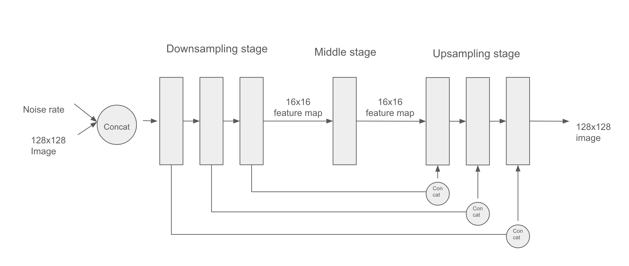
This architecture features three stages:
- A downsampling stage, consisting of several blocks of convolution layers, where the inputs are downsampled from their original 128 × 128 size to a much smaller size (in our case, 16 × 16)
- A middle stage where the feature map has a constant size
- An upsampling stage, where the feature map is upsampled back to 128 × 128
There is a 1:1 mapping between the blocks of the downsampling and upsampling stages: each upsampling block is the inverse of a downsampling block. Importantly, the model features concatenative residual connections going from each downsampling block to the corresponding upsampling block. These connections help avoid loss of image detail information across the successive downsampling and upsampling operations.
Let’s assemble the model using the Functional API:
1residual_block <- function(x, width) {
  .[.., n_features] <- op_shape(x)

  if (n_features == width) {
    residual <- x
  } else {
    residual <- x |> layer_conv_2d(filters = width, kernel_size = 1)
  }

  x <- x |>
    layer_batch_normalization(center = FALSE, scale = FALSE) |>
    layer_conv_2d(width, kernel_size = 3, padding = "same",
                  activation = "swish") |>
    layer_conv_2d(width, kernel_size = 3, padding = "same")

  x + residual
}


get_model <- function(image_size, widths, block_depth) {
  noisy_images <- keras_input(shape = c(image_size, image_size, 3))
  noise_rates <- keras_input(shape = c(1, 1, 1))

  x <- noisy_images |> layer_conv_2d(filters = widths[1], kernel_size = 1)
  n <- noise_rates |>
    layer_upsampling_2d(size = image_size, interpolation = "nearest")
  x <- layer_concatenate(c(x, n))

  skips <- list()

2  for (width in head(widths, -1)) {
    for (i in seq_len(block_depth)) {
      x <- x |> residual_block(width)
      skips <- c(skips, x)
    }
    x <- x |> layer_average_pooling_2d(pool_size = 2)
  }

3  for (i in seq_len(block_depth)) {
    x <- x |> residual_block(tail(widths, 1))
  }

4  for (width in rev(head(widths, -1))) {
    x <- x |> layer_upsampling_2d(size = 2, interpolation = "bilinear")
    for (i in seq_len(block_depth)) {
      x <- x |> layer_concatenate(tail(skips, 1)[[1]])
      skips <- head(skips, -1)
      x <- x |> residual_block(width)
    }
  }

5  pred_noise_masks <- x |> layer_conv_2d(
    filters = 3, kernel_size = 1, kernel_initializer = "zeros"
  )

6  model <- keras_model(inputs = list(noisy_images, noise_rates),
                       outputs = pred_noise_masks)
  model
}- 1
- Utility function to apply a block of layers with a residual connection
- 2
- Downsampling stage
- 3
- Middle stage
- 4
- Upsampling stage
- 5
-
We set the kernel initializer for the last layer to
zeros, making the model predict only zeros after initialization (that is, our default assumption before training is “no noise”). - 6
- Creates the functional model
We would instantiate the model with something like get_model(image_size=128, widths=c(32, 64, 96, 128), block_depth=2). The widths argument is a list containing the Conv2D layer sizes for each successive downsampling or upsampling stage. We typically want the layers to get bigger as we downsample the inputs (going from 32 to 128 units here) and then get smaller as we upsample (from 128 back to 32 here).
17.2.3 The concepts of diffusion time and diffusion schedule
The diffusion process is a series of steps in which we apply our denoising autoencoder to erase a small amount of noise from an image, starting with a pure-noise image and ending with a pure-signal image. The index of the current step in the loop is called the diffusion time (see figure 17.7). In our case, we’ll use a continuous value between 0 and 1 for this index—a value of 1 indicates the start of the process, where the amount of noise is maximal, and the amount of signal is minimal, and a value of 0 indicates the end of the process, where the image is almost all signal and no noise.
The relationship between the current diffusion time and the amount of noise and signal present in the image is called the diffusion schedule. In our experiment, we’ll use a cosine schedule to smoothly transition from a low signal rate (high noise) at the beginning to a high signal rate (low noise) at the end of the diffusion process.
diffusion_schedule <- function(diffusion_times, min_signal_rate = 0.02,
max_signal_rate = 0.95) {
start_angle <- op_arccos(max_signal_rate) |> op_cast(dtype = "float32")
end_angle <- op_arccos(min_signal_rate) |> op_cast(dtype = "float32")
diffusion_angles <-
start_angle + diffusion_times * (end_angle - start_angle)
signal_rates <- op_cos(diffusion_angles)
noise_rates <- op_sin(diffusion_angles)
list(noise_rates = noise_rates, signal_rates = signal_rates)
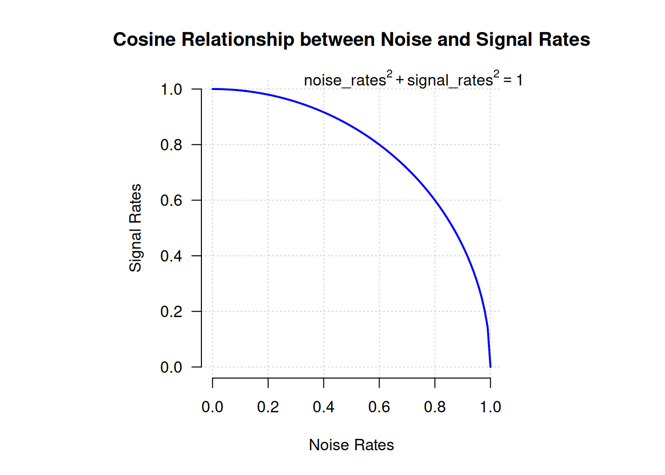
}This diffusion_schedule() function takes as input a diffusion_times tensor, which represents the progression of the diffusion process and returns the corresponding noise_rates and signal_rates tensors. These rates will be used to guide the denoising process. The logic behind using a cosine schedule is to maintain the relationship noise_rates^2 + signal_rates^2 == 1 (see figure 17.10).
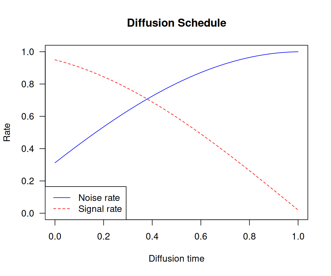
Let’s plot how this function maps diffusion times (between 0 and 1) to specific noise rates and signal rates (see figure 17.11):
1diffusion_times <- op_arange(0, 1, 0.01)
schedule <- diffusion_schedule(diffusion_times)

2diffusion_times <- as.array(diffusion_times)
noise_rates <- as.array(schedule$noise_rates)
signal_rates <- as.array(schedule$signal_rates)

3plot(NULL, type = "n", main = "Diffusion Schedule",
     ylab = "Rate",  ylim = c(0, 1),
     xlab = "Diffusion time", xlim = c(0, 1))
4lines(diffusion_times, noise_rates, col = "blue", lty = 1)
lines(diffusion_times, signal_rates, col = "red", lty = 2)

5legend("bottomleft",
       legend = c("Noise rate", "Signal rate"),
col = c("blue", "red"), lty = c(1, 2))- 1
- Generates diffusion times and computes the cosine schedule
- 2
- Converts tensors to R numeric vectors
- 3
- Sets up an empty plot
- 4
- Plots the noise and signal rates
- 5
- Adds a legend to label the lines
17.2.4 The training process
Let’s create a DiffusionModel class to implement the training procedure. It will have our denoising autoencoder as one of its attributes. We also need a couple more things:
- A loss function—We’ll use mean absolute error as our loss:
mean(abs(real_noise_mask - predicted_noise_mask)). - An image normalization layer—The noise we’ll add to the images will have unit variance and zero mean, so we’d like our images to be normalized as such too, for the value range of the noise to match the value range of the images.
Let’s start by writing the model constructor:
new_diffusion_model <- new_model_class(
  classname = "DiffusionModel",

  initialize = function(image_size, widths, block_depth, ...) {
    super$initialize(...)
    self$image_size <- shape(image_size)
    self$denoising_model <- get_model(image_size, widths, block_depth)
    self$seed_generator <- random_seed_generator()
1    self$loss <- loss_mean_absolute_error()
2    self$normalizer <- layer_normalization()
},- 1
- Our loss function
- 2
- We’ll use this to normalize input images
The first method we’ll need is the denoising method. It simply calls the denoising model to retrieve a predicted noise mask, which it uses to reconstruct a denoised image:
- 1
- Calls the denoising model
- 2
- Reconstructs the predicted clean image
Next, here’s the training logic. This is the most important part! As in the VAE example, we’ll implement a custom compute_loss() method to keep our model backend-agnostic. Of course, if you are set on using one specific backend, you can also write a custom train_step() with the exact same logic in it, plus the backend-specific logic for gradient computation and weight updates.
Because compute_loss() receives as input the output of call(), we’ll put the denoising forward pass in call(). Our call() takes a batch of clean input images and applies the following steps:
- Normalizes the images
- Samples random diffusion times (the denoising model needs to be trained on the full spectrum of diffusion times)
- Computes corresponding noise rates and signal rates (using the diffusion schedule)
- Adds random noise to the clean images (based on the computed noise rates and signal rates)
- Denoises the images
It returns
- The predicted denoised images
- The predicted noise masks
- The actual noise masks it applied
These last two quantities are then used in compute_loss() to compute the loss of the model on the noise mask prediction task:
  call = function(images) {
    images <- self$normalizer(images)
    .[batch_size, ..] <- op_shape(images)

1    noise_masks <- random_normal(
      shape = c(batch_size, self$image_size, self$image_size, 3),
      seed = self$seed_generator
    )

2    diffusion_times <- random_uniform(
      shape = c(batch_size, 1, 1, 1),
      minval = 0.0, maxval = 1.0,
      seed = self$seed_generator
    )

    .[noise_rates, signal_rates] <- diffusion_schedule(diffusion_times)
3    noisy_images <- signal_rates * images + noise_rates * noise_masks

    .[pred_images, pred_noise_masks] <-
4      self$denoise(noisy_images, noise_rates, signal_rates)

    list(pred_images, pred_noise_masks, noise_masks)
  },

  compute_loss = function(x, y, y_pred,
                          sample_weight = NULL,
                          training = TRUE) {
    .[.., pred_noise_masks, noise_masks] <- y_pred
    self$loss(noise_masks, pred_noise_masks)
},- 1
- Samples random noise masks
- 2
- Samples random diffusion times
- 3
- Adds noise to the images
- 4
- Denoises them
17.2.5 The generation process
Finally, let’s implement the image generation process. We start from pure random noise, and we repeatedly apply the denoise() method until we get high-signal, low-noise images.
  generate = function(num_images, diffusion_steps) {
1    noisy_images <- random_normal(
      shape = c(num_images, self$image_size, self$image_size, 3),
      seed = self$seed_generator
    )

    diffusion_times <- seq(1, 0, length.out = diffusion_steps)

    for (i in seq_len(diffusion_steps - 1)) {
      diffusion_time <- diffusion_times[i]
      next_diffusion_time <- diffusion_times[i + 1]

      .[noise_rates, signal_rates] <- diffusion_time |>
        op_broadcast_to(c(num_images, 1, 1, 1)) |>
2        diffusion_schedule()

3      .[pred_images, pred_noises] <-
        self$denoise(noisy_images, noise_rates, signal_rates)

      .[next_noise_rates, next_signal_rates] <- next_diffusion_time |>
        op_broadcast_to(c(num_images, 1, 1, 1)) |>
4        diffusion_schedule()

      noisy_images <-
        (next_signal_rates * pred_images) +
        (next_noise_rates * pred_noises)
    }

    images <-
5      self$normalizer$mean + pred_images * op_sqrt(self$normalizer$variance)

    op_clip(images, 0, 255)
  }
)- 1
- Starts from pure noise
- 2
- Computes appropriate noise rates and signal rates
- 3
- Calls the denoising model
- 4
- Prepares noisy images for the next iteration
- 5
- Denormalizes the images so their values fit between 0 and 255
17.2.6 Visualizing results with a custom callback
We don’t have a proper metric to judge the quality of our generated images, so we want to visualize the generated images over the course of training to judge whether the model is improving. An easy way to do this is with a custom callback. The following callback uses the generate() method at the end of each epoch to display a 3 × 6 grid of generated images:
callback_visualization <- new_callback_class(
  classname = "VisualizationCallback",
  initialize = function(diffusion_steps = 20, num_rows = 3, num_cols = 6) {
    self$diffusion_steps <- diffusion_steps
    self$num_rows <- num_rows
    self$num_cols <- num_cols
  },

  on_epoch_end = function(epoch = NULL, logs = NULL) {
    generated_images <- self$model$generate(
      num_images = self$num_rows * self$num_cols,
      diffusion_steps = self$diffusion_steps
    ) |> as.array()

    par(mfrow = c(self$num_rows, self$num_cols),
        mar = c(0, 0, 0, 0))

    for (i in seq_len(self$num_rows * self$num_cols))
      plot(as.raster(generated_images[i, , , ], max = 255))

  }
)
17.2.7 It’s go time!
It’s finally time to train our diffusion model on the Oxford Flowers dataset. Let’s instantiate the model:
model <- new_diffusion_model(
  image_size,
  widths = c(32, 64, 96, 128),
  block_depth = 2
)
1model$normalizer$adapt(dataset)- 1
- Computes the mean and variance necessary to perform normalization—don’t forget it!
We’ll use AdamW as our optimizer, with a few neat options enabled to help stabilize training and improve the quality of the generated images:
- Learning-rate decay—We gradually reduce the learning rate during training, via an
InverseTimeDecayschedule. - Exponential moving average of model weights—Also known as Polyak averaging. This technique maintains a running average of the model’s weights during training. Every 100 batches, we overwrite the model’s weights with this averaged set of weights. This helps stabilize the model’s representations in scenarios where the loss landscape is noisy.
The code is as follows:
- 1
- Configures the learning rate decay schedule
- 2
- Turns on Polyak averaging
- 3
- Configures how often to overwrite the model’s weights with their exponential moving average
Let’s fit the model. We’ll use our VisualizationCallback to plot examples of generated images after each epoch, and we’ll save the model’s weights with the ModelCheckpoint callback:
model |> fit(
  dataset,
  epochs = 100,
  callbacks = list(
    callback_visualization(),
    callback_model_checkpoint(
      filepath = "diffusion_model.weights.h5",
      save_weights_only = TRUE,
      save_best_only = TRUE,
      monitor = "loss"
    )
  )
)
Note
If you’re running on Colab, you might run into the error “Buffered data was truncated after reaching the output size limit.” This happens because the logs of fit() include images, which take up a lot of space, whereas the output allowed for a single notebook cell is limited. To get around the problem, you can simply chain five model |> fit(..., epochs=20) calls in five successive cells. This is equivalent to a single fit(..., epochs=100) call.
After 100 epochs (which takes about 90 minutes on a T4, the free Colab GPU), we get pretty generative flowers like those shown in figure 17.12. You can keep training even longer and get increasingly realistic results.
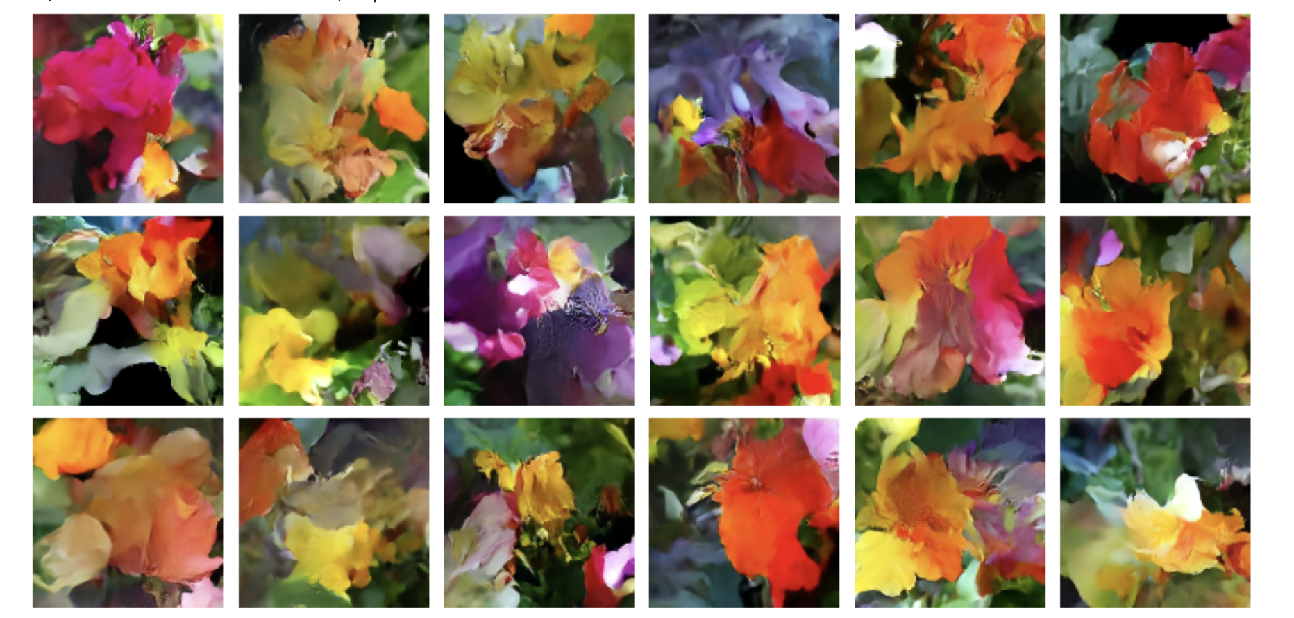
So that’s how image generation with diffusion works! The next step to unlock its potential is to add text conditioning, which results in a text-to-image model that can produce images that match a given text caption.
17.3 Text-to-image models
We can use the same basic diffusion process to create a model that maps text input to image output. To do this, we need to take a pretrained text encoder (think a transformer encoder like RoBERTa from chapter 15) that can map text to vectors in a continuous embedding space. Then we can train a diffusion model on (prompt, image) pairs, where each prompt is a short, textual description of the input image.
We can handle the image input the same way we did previously, mapping noisy input to a denoised output that progressively approaches our input image. Critically, we can extend this setup by also passing the embedded text prompt to the denoising model. So rather than our denoising model simply taking a noisy_images input, our model will take two inputs: noisy_images and text_embeddings. This gives it a leg up on the flower denoiser we trained previously. Instead of learning to remove noise from an image without any additional information, the model gets to use a textual representation of the final image to help guide the denoising process.
After training, things get more fun. Because we have trained a model that can map pure noise to images conditioned on a vector representation of some text, we can pass in pure noise and a never-before-seen prompt and denoise it into an image for our prompt.
Let’s try this out. We won’t actually train one of these models from scratch in this book—you have all the ingredients you need, but it’s quite expensive and time-consuming to train a text-to-image diffusion model that works well. Instead, we will play with a popular pretrained model in KerasHub called Stable Diffusion (figure 17.13). Stable Diffusion is made by a company named Stability AI that specializes in making open models for image and video generation. We can use the third version of their image generation model in KerasHub with just a couple of lines of code:
library(keras3)
py_require("keras-hub")
keras_hub <- import("keras_hub")

.[height, width] <- c(512, 512)
task <- keras_hub$models$TextToImage$from_preset(
  "stable_diffusion_3_medium",
  image_shape = shape(height, width, 3),
1  dtype = "float16"
)
prompt <- "A NASA astronaut riding an origami elephant in New York City"- 1
- A trick to keep down memory usage. More details in Chapter 18.
image <- task$generate(prompt)
par(mar = c(0, 0, 0, 0))
plot(as.raster(image, max = max(image)))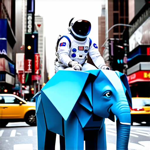
Like the CausalLM task we covered in the last chapter, the TextToImage task is a high-level class for performing image generation conditioned on text input. It wraps tokenization and the diffusion process into a high-level generate call.
The Stable Diffusion model actually adds a second “negative prompt” to its model, which can be used to steer the diffusion process away from certain text inputs. There’s nothing magic here. To support negative prompts, we can train a model on triplets: (image, positive_prompt, negative_prompt), where the positive prompt is a description of the image and the negative prompt is a series of words that do not describe the image. At generation time, we feed both the positive and negative text embeddings to the denoiser, and the denoiser uses them to steer the noise toward images that match the positive prompt and away from images that match the negative prompt (figure 17.14). Let’s try removing the color blue from our input:
image <- task$generate(list(
  prompts = prompt,
  negative_prompts = "blue color"
))
par(mar = c(0, 0, 0, 0))
plot(as.raster(image, max = max(image)))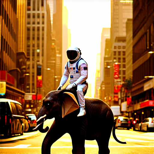
NoteVisual artifacts in the Stable Diffusion output
You will notice plenty of visual artifacts in our Stable Diffusion output if you look closely. Notably, our second elephant has duplicated tusks!
Some of this is unavoidable when using diffusion models. Figuring out how to truly draw a human in a space suit sitting on an elephant made of paper would require some understanding of anatomy and physics that our model lacks. The model will always try its best to interpolate an output based on its training data, but it doesn’t have any real understanding of the objects it is attempting to represent.
However, there is another factor that is easily fixable: we are using the less-powerful version of Stable Diffusion 3. The “medium” model we are using is the smallest one released by Stability AI and uses about 3 billion parameters in total. There is a larger, 9-billion-parameter model available that would produce substantially higher-quality images with fewer visual artifacts. We do not use it simply to keep the code example in this book accessible—9 billion parameters need a lot of RAM!
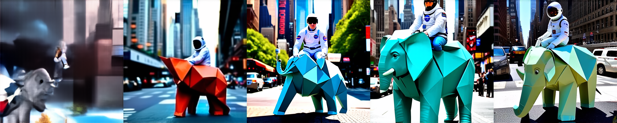
As with the generate() method for text models that we used in the last chapter, we can pass a few additional parameters to control the generation process. Let’s try passing a variable number of diffusion steps to our model to see the denoising process in action (figure 17.15):
par(mfrow = c(1, 5), mar = c(0, 0, 0, 0))
for (num_steps in c(5, 10, 15, 20, 25)) {
  image <- task$generate(prompt, num_steps = num_steps)
  plot(as.raster(image, max = max(image)))
}
17.3.1 Exploring the latent space of a text-to-image model
There is probably no better way to see the interpolative nature of deep neural networks than text diffusion models. The text encoder used by our model will learn a smooth, low-dimensional manifold to represent our input prompts. It’s continuous, meaning we have learned a space where we can walk from the text representation of one prompt to another, and each intermediate point will have semantic meaning. We can couple that with our diffusion process to morph between two images by simply describing each end state with a text prompt.
Before we can do this, we will need to break up our high-level generate() function into its constituent parts. Let’s try that out.
generate() function
get_text_embeddings <- function(prompt) {
  token_ids <- task$preprocessor$generate_preprocess(list(prompt))
1  negative_token_ids <- task$preprocessor$generate_preprocess(list(""))
  task$backbone$encode_text_step(token_ids, negative_token_ids)
}

denoise_with_text_embeddings <- function(
  embeddings,
  num_steps = 28L,
  guidance_scale = 7
) {
2  latents <- random_normal(c(1, height %/% 8, width %/% 8, 16))
  for (step in seq_len(num_steps)) {
    latents <- latents |>
      task$backbone$denoise_step(
        embeddings, step, num_steps, guidance_scale
      )
  }
  task$backbone$decode_step(latents)@r[1]
}


scale_output <- function(x) {
3  op_clip((x + 1) / 2, 0, 1)
}

embeddings <- get_text_embeddings(prompt)
image <- denoise_with_text_embeddings(embeddings)
image <- scale_output(image)- 1
- We don’t care about negative prompts here, but the model expects them.
- 2
- Creates pure noise to denoise into an image
- 3
- Rescales our images back to [0, 1]
par(mar = c(0,0,0,0))
plot(as.raster(as.array(image)))
The result is shown in figure 17.16.
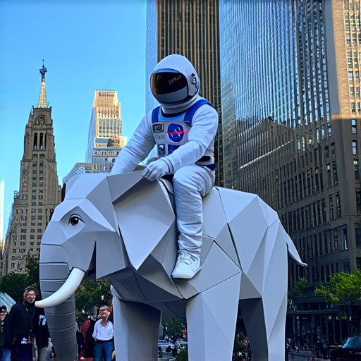
Our generation process has three distinct parts:
- Tokenize our prompts and embed them with our text encoder.
- Take our text embeddings and pure noise and progressively “denoise” the noise into an image. This is the same as the flower model we just built.
- Map our model output, which is from
[-1, 1]back to[0, 1]so we can render the image.
One thing to note here is that our text embeddings actually contain four separate tensors:
str(embeddings)List of 4
$ : <jax.Array shape(1, 154, 4096), dtype=float16>
$ : <jax.Array shape(1, 154, 4096), dtype=float16>
$ : <jax.Array shape(1, 2048), dtype=float16>
$ : <jax.Array shape(1, 2048), dtype=float16>Rather than passing only the final, embedded text vector to the denoising model, the Stable Diffusion authors chose to pass both the final output vector and the last representation of the entire token sequence learned by the text encoder. This effectively gives our denoising model more information to work with. The authors do this for both the positive and negative prompts, so we have a total of four tensors here:
- The positive prompt’s encoder sequence
- The negative prompt’s encoder sequence
- The positive prompt’s encoder vector
- The negative prompt’s encoder vector
With our generate() function decomposed, we can now try walking the latent space between two text prompts. To do so, let’s build a function to interpolate between the text embeddings outputted by the model.
slerp <- function(t, v1, v2) {
  .[v1, v2] <- list(v1, v2) |> lapply(op_cast, "float32")
  v1_norm  <- op_norm(op_ravel(v1))
  v2_norm  <- op_norm(op_ravel(v2))
  dot <- op_sum(v1 * v2 / (v1_norm * v2_norm))
  theta_0 <- op_arccos(dot)
  sin_theta_0 <- op_sin(theta_0)
  theta_t <- theta_0 * t
  sin_theta_t <- op_sin(theta_t)
  s0 <- op_sin(theta_0 - theta_t) / sin_theta_0
  s1 <- sin_theta_t / sin_theta_0
  s0 * v1 + s1 * v2
}

interpolate_text_embeddings <- function(e1, e2, start=0, end=1, num=10) {
  lapply(seq(start, end, length.out = num), \(t) {
    list(
      slerp(t, e1[[1]], e2[[1]]),
1      e1[[2]],
      slerp(t, e1[[3]], e2[[3]]),
      e1[[4]]
    )
  })

}- 1
- The second and fourth text embeddings are for the negative prompt, which we do not use.
You’ll notice that we use a special interpolation function called slerp to walk between our text embeddings. This is short for spherical linear interpolation—it’s a function that has been used in computer graphics for decades to interpolate points on a sphere.
Don’t worry too much about the math; it’s not important for our example, but it is important to understand the motivation. If we imagine our text manifold as a sphere and our two prompts as random points on that sphere, directly linearly interpolating between these two points would land us inside the sphere. We would no longer be on its surface. We would like to stay on the surface of the smooth manifold learned by our text embedding: that’s where embedding points have meaning for our denoising model. See figure 17.17.
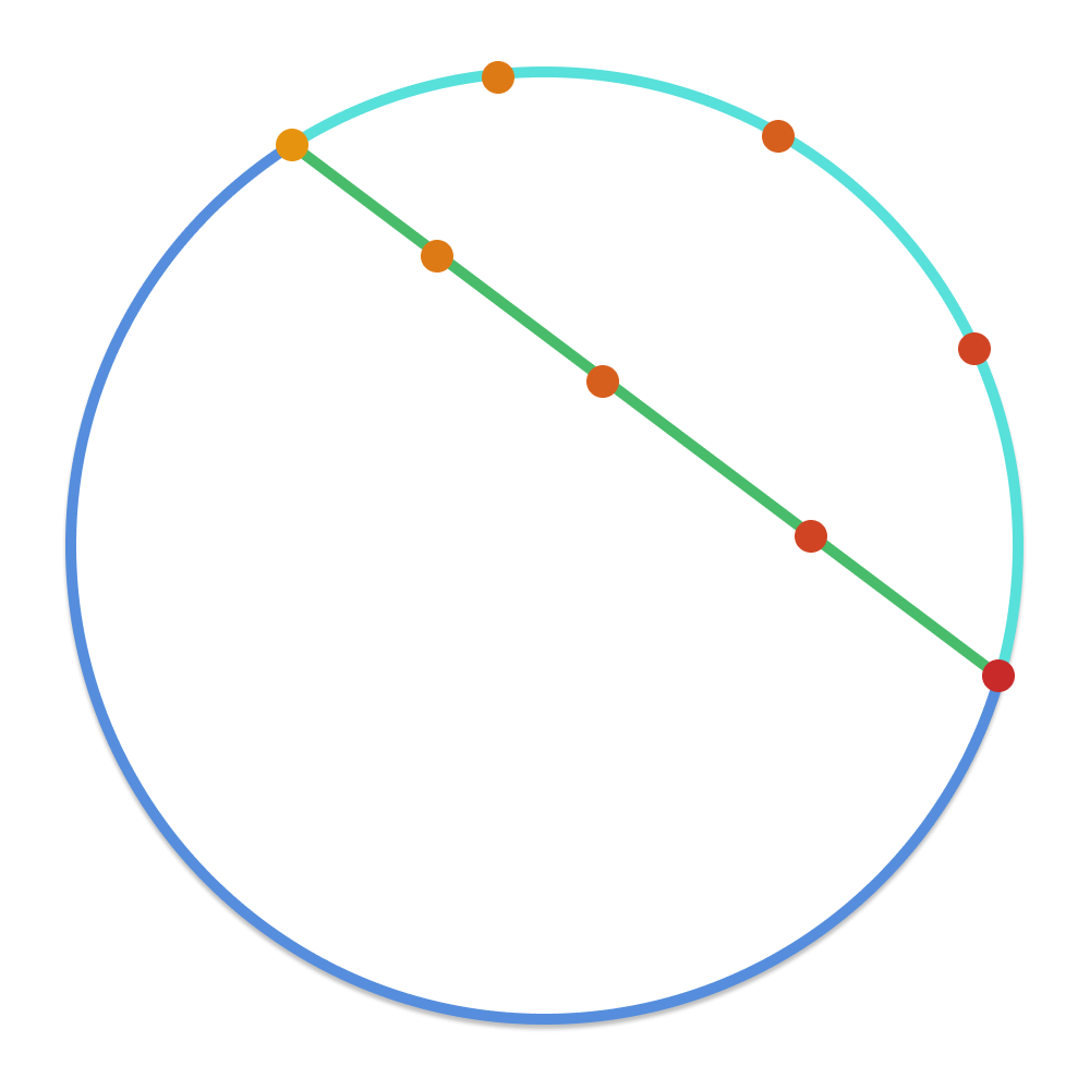
Of course, the manifold learned by our text embedding model is not actually spherical. But it’s a smooth surface of numbers all with the same rough magnitude—it is sphere-like, and interpolating as if we were on a sphere is a better approximation than interpolating as if we were on a line.
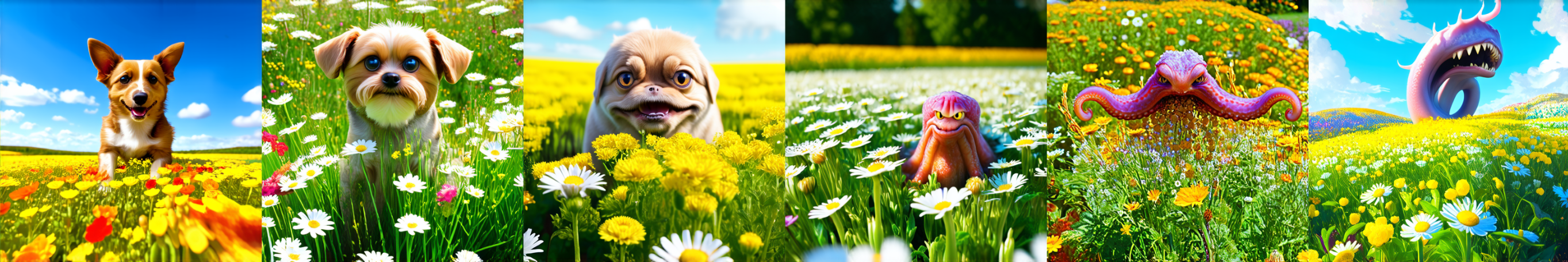
With our interpolation defined, let’s try walking between the text embeddings for two prompts and generating an image at each interpolated output. We will run our slerp function from 0.5 to 0.6 (out of 0 to 1) to zoom in on the middle of the interpolation right when the “morph” becomes visually obvious (figure 17.18):
par(mar = c(0,0,0,0))
prompt1 <- "A friendly dog looking up in a field of flowers"
prompt2 <- "A horrifying, tentacled creature hovering over a field of flowers"
e1 <- get_text_embeddings(prompt1)
e2 <- get_text_embeddings(prompt2)

1for (et in interpolate_text_embeddings(e1, e2, start=0.5, end=0.6, num=9)) {
  image <- denoise_with_text_embeddings(et)
  plot(as.raster(as.array(scale_output(image))))
}- 1
- Zooms in to the middle of the overall interpolation from [0, 1]
This may feel like magic the first time you try it, but there’s nothing magic about it—interpolation is fundamental to the way deep neural networks learn. This will be the last substantive model we work with in the book, and it’s a great visual metaphor to end with. Deep neural networks are interpolation machines; they map complex, real-world probability distributions to low-dimensional manifolds. We can exploit this fact even for input as complex as human language and output as complex as natural images.
17.4 Summary
Image generation with deep learning is done by learning latent spaces that capture statistical information about a dataset of images. By sampling and decoding points from the latent space, you can generate never-before-seen images. There are three major tools to do this: VAEs, diffusion models, and GANs.
VAEs result in highly structured, continuous latent representations. For this reason, they work well for doing all sorts of image editing in latent space: face swapping, turning a frowning face into a smiling face, and so on. They also work nicely for doing latent space-based animations, such as animating a walk along a cross-section of the latent space, showing a starting image slowly morphing into different images in a continuous way.
Diffusion models result in very realistic outputs and are the dominant method of image generation today. They work by repeatedly denoising an image, starting from pure noise. They can easily be conditioned on text captions to create text-to-image models.
Stable Diffusion 3 is a state-of-the-art pretrained text-to-image model that you can use to create highly realistic images of your own.
The visual latent space learned by such text-to-image diffusion models is fundamentally interpolative. You can see this by interpolating between the text embeddings used as inputs to the diffusion process and achieving a smooth interpolation between images as output.
Diederik P. Kingma and Max Welling, “Auto-Encoding Variational Bayes,” arXiv (2013), https://arxiv.org/abs/1312.6114.↩︎
Danilo Jimenez Rezende, Shakir Mohamed, and Daan Wierstra, “Stochastic Backpropagation and Approximate Inference in Deep Generative Models,” arXiv (2014), https://arxiv.org/abs/1401.4082.↩︎